Vildagliptin GLP-1 / glucose / insulin systems model (Landersdorfer 2012)
Source:vignettes/articles/Landersdorfer_2012_vildagliptin_qsp.Rmd
Landersdorfer_2012_vildagliptin_qsp.RmdModel and source
mod <- readModelDb("Landersdorfer_2012_vildagliptin_qsp")
ui  <- rxode2::rxode(mod)
#> ℹ parameter labels from comments will be replaced by 'label()'- Citation: Landersdorfer CB, He YL, Jusko WJ. Mechanism-based population modelling of the effects of vildagliptin on GLP-1, glucose and insulin in patients with type 2 diabetes. Br J Clin Pharmacol. 2012;73(3):373-390. doi:10.1111/j.1365-2125.2011.04109.x. PMCID: PMC3370342. The vildagliptin PK and DPP-4 layer is the companion report: Landersdorfer CB, He YL, Jusko WJ. Mechanism-based population pharmacokinetic modelling in diabetes: vildagliptin as a tight binding inhibitor and substrate of dipeptidyl peptidase IV. Br J Clin Pharmacol. 2012;73(3):391-401. doi:10.1111/j.1365-2125.2011.04108.x; see modellib(‘Landersdorfer_2012_vildagliptin’).
- Article: https://doi.org/10.1111/j.1365-2125.2011.04109.x (PMC3370342, open access)
- Companion PK / DPP-4 article: https://doi.org/10.1111/j.1365-2125.2011.04108.x
(packaged separately as
modellib("Landersdorfer_2012_vildagliptin"))
This is the pharmacodynamic half of a companion pair. The companion article describes vildagliptin PK and DPP-4 activity as a target-mediated drug disposition (TMDD) model; the present article adds three downstream endpoints – active GLP-1, plasma glucose and plasma insulin – and states that “in the full PK/PD model all PK (shown in the companion report) and PD parameters were estimated at the same time” (Methods, p. 376). The whole system is therefore one jointly-fitted model and is packaged as one file.
Population
13 adults with type 2 diabetes mellitus diagnosed at least three months before screening, after a washout from hypoglycaemic drugs of up to four weeks. Mean (range) weight 91 (65-116) kg, height 166 (148-183) cm, age 53.5 (37-64) years; seven female and six male (Results, first paragraph). The design was a randomized, double-blind, placebo-controlled four-way crossover: oral vildagliptin 10, 25 or 100 mg twice daily for 28 days, plus placebo. Twelve subjects completed all four periods and one completed only the 10 and 25 mg treatments. Patients were confined from the evening of day 26 to the morning of day 29 of each period and received a standard diet with identical meals across all four treatments (55% carbohydrate, 25% fat, 20% protein). GLP-1, glucose and insulin were sampled on day 28.
The same information is available programmatically via
readModelDb("Landersdorfer_2012_vildagliptin_qsp")()$population.
Errata and non-paper-derived values
Two quantities the model needs are not usable as printed. Both are resolved below from the paper’s own figures; read this section before using the model.
1. V_glc is not reported anywhere
The glucose ODE divides the gut absorption rate by a volume of
distribution of glucose,
Glc_GutAb = (k_aB*A_GB + k_aL*A_GL + k_aD*A_GD + k_aS*A_GS) / V_glc.
The Methods define the symbol – “where Vglc (dl) is the volume of
distribution of glucose” (p. 376) – and then never give a value: it is
absent from Table 1, from the body text, from Figure 1, from the
companion article, and there is no supplement and no erratum.
It does not cancel out. The meal-amount scale is pinned independently
by the GLP-1 arm (S1 is reported in g^-1 and multiplies
Glc_Gut), so V_glc is a free constant that
sets the magnitude of every glucose excursion and, through the
glucose-insulin feedback, the insulin profile too.
Per maintainer ruling (2026-09-02) it was back-solved from
the Figure 3 placebo panel: the published median curve was
digitised and V_glc fitted to it, giving 250 dL
(25.0 L). Ninety-six combinations of the unreported meal times
and food-intake durations bracket the estimate at 246-255 dL, so the
value is set by the glucose level rather than by the timing
assumptions.
Two independent consequences, neither used in the fit, support it:
- endogenous glucose production
B_glc * k_out_glc * V_glc= 11.1 g/h = 2.0 mg/kg/min at the cohort’s mean 91 kg, the textbook human value; - the resulting typical-value profile also reproduces Figure 7A-D (below), which the fit never saw.
The glucose validation against Figure 3 is therefore partly circular and is labelled as such below; the Figure 2, 4 and 7 comparisons are not.
2. S5 is printed with a lost unit prefix
Table 1 gives S5 = 0.584 with units
l mIU-1. Taken literally the model cannot reproduce any of
the paper’s own figures – glucose elimination at a postprandial peak
would be roughly 40 h^-1, a glucose half-life near one minute – and the
best-fitting V_glc becomes 2 dL, a physiological
impossibility.
Figure 7B settles it directly. That panel plots
ST_ins = S5 * [1 + S4 * (C_glp - B_glp)] against time on a
0 to 0.009 axis, and at baseline GLP-1 the bracket is
exactly 1, so the panel reads S5 off its own y-axis. The
published 0.584 l mIU-1 is 640-fold above the top
of that axis; 5.84e-4 l mIU-1 =
0.584 mL/mIU sits on the placebo curve’s fasting value of
about 0.001. The paper drops a unit prefix on this pair of quantities
elsewhere too: the Results section (p. 377) prints ST_glc
as l mg-1 where Table 1 and dimensional analysis both
require dl mg-1.
The model file keeps the printed 0.584 in
ini() and applies an explicit mL -> L
conversion in model(), so the published number stays
visible and the correction is auditable on one line.
No other parameter needed adjustment: Figure 7C confirms
S3 = 0.0185 dl mg-1 on its own axis, Figure 7A confirms
R_maxC * cf2 = 3.2 h^-1, and the Discussion’s “increase in
insulin secretion of 35% for a 5 pmol l-1 increase in GLP-1” reproduces
exactly from S2 (checked below).
Source trace
Every ini() entry carries an in-file comment naming its
source location; the table collects them.
| Parameter / equation | Value | Source location |
|---|---|---|
lka1, lka2, lcl,
lvc, lvp, lq
|
1.26, 1.05 /h; 36.4 L/h; 22.2, 97.3 L; 40.1 L/h | Companion (04108.x) Table 1 |
lfdepot |
0.772 (fixed) | Companion Table 1, footnote * |
lkd, lk2, lkoff,
lkdeg
|
71.9 nmol/L; 23.4, 0.612, 0.110 /h | Companion Table 1 |
lrmaxc, lrmaxp, lcf1
|
5.0, 13000 nmol; 2.80 | Companion Table 1 (R_maxP printed “13.0 mmol”; see
below) |
lkout_glp_lin, ls1, lcf2,
lbl_glp
|
2.07 /h; 0.049 /g; 0.641; 1.68 pmol/L | Table 1, p. 380 |
lfdepot_breakfast/lunch/dinner/snack |
0.796, 0.865, 0.817, 0.342 | Table 1 (F_B, F_L, F_D,
F_S) |
lka_breakfast/lunch/dinner/snack |
0.732, 0.520, 0.252, 0.169 /h | Table 1 (k_aB, k_aL, k_aD,
k_aS) |
lbl_glc, lkout_glc, ls5,
ls4
|
133 mg/dL; 0.334 /h; 0.584 mL/mIU; 1.90 L/pmol | Table 1 (S5 prefix per Figure 7B) |
lv_glc |
250 dL | Not published – back-solved from Figure 3 |
lbl_ins, lkout_ins, ls3,
ls2
|
9.75 mIU/L; 14.0 /h; 0.0185 dL/mg; 0.0701 L/pmol | Table 1 |
| IIV (all etas) | BSV% squared | Table 1 “BSV (%)”; S-ADAPT reports sqrt(variance) (Methods p. 376) |
| Residual error (5 outputs) |
CV/SD pairs |
Table 1 (PD) and companion Table 1 (PK) |
Meal gut ODEs, Glc_Gut
|
n/a | Methods “Structural PD model”, p. 375 |
GLP-1 ODE, k_in_glp steady state |
n/a | Methods p. 376 |
Glc_GutAb, glucose ODE, insulin ODE,
ST_ins, ST_glc
|
n/a | Methods p. 376 |
Two printed-unit problems were resolved from internal evidence and are recorded in the model file next to the affected line:
-
S1– Table 1 givesg-1, the body text (p. 376) givesmg-1. Table 1 is right: withS1 = 0.049 mg-1a ~50 g meal bolus would stimulate GLP-1 secretion ~2450-fold. Gut amounts are therefore carried in grams. -
R_maxP– the companion Table 1 prints “13.0 mmol”; 13 umol / 5 nmol = 2600-fold matches that paper’s own “>2000-fold” tissue:plasma statement, whereas 13 mmol would be 2.6e6-fold and about 1.4 kg of a 110 kDa enzyme.
Reconstructing the study day
The paper gives the meal structure but not the full timetable. What
is stated: meals were standardised and identical across periods;
“breakfast and dinner were consumed at approximately 30 min after the
doses” (Methods, p. 374); the evening dose was at 10.5 h (from the
sampling schedule); and the input duration tk0 was “the
actual recorded duration of food intake for each individual patient and
each meal”, which is never reported. Lunch and snack times are not
given.
Lunch and snack are recovered from the published figures: Figures 2,
3, 4 and 7 all show four meal-driven excursions per day, spaced about
5.1, 5.4 and 3.5 h apart. The schedule below combines the stated design
with those spacings, and tk0 is assumed to be 45 min.
V_glc moves by less than 4% across the whole grid of
plausible alternatives, so nothing downstream hinges on it.
MEAL_TIMES <- c(breakfast = 0.5, lunch = 5.6, dinner = 11.0, snack = 14.5)
TK0        <- 0.75   # h; duration of food intake (assumed -- not reported)
MEAL_G     <- 75     # g; the paper's arbitrary 75000 mg per-meal anchor
DOSE_TIMES <- c(0, 10.5)
N_DAY      <- 5L     # days of BID dosing simulated before the observed day
ARMS       <- c(Placebo = 0, `10 mg` = 10, `25 mg` = 25, `100 mg` = 100)
# One arm's event table. Observation records name an ENDPOINT (Cglc). This
# model declares five endpoints, so rxode2 requires observation rows to select
# among the endpoint slots; naming one does NOT renumber the ODE states (they
# keep slots 1-13) and every observable still comes back as its own column.
# The same idiom is used by the sibling Landersdorfer_2012_vildagliptin and by
# Bosch_2024_cotadutide_qsp vignettes.
# `obs` is a parameter rather than hard-coded because observation times MUST be
# added while the table is still an `rxEt`. Passing an already-materialized
# data.frame back into `rxode2::et()` and asking for extra sampling times
# silently DROPS them -- no error, no warning -- which makes any downstream
# `x[time %in% ...]` selection empty and any `stopifnot()` over it pass
# vacuously.
build_arm <- function(dose_mg, id,
                      obs = seq(24 * (N_DAY - 1L), 24 * N_DAY, by = 0.05)) {
  ev <- rxode2::et(id = id)
  for (d in seq_len(N_DAY) - 1L) {
    if (dose_mg > 0) {
      for (dt in DOSE_TIMES) {
        ev <- rxode2::et(ev, id = id, amt = dose_mg, cmt = "depot", time = 24 * d + dt)
      }
    }
    for (m in names(MEAL_TIMES)) {
      ev <- rxode2::et(ev, id = id, amt = MEAL_G, dur = TK0,
                       cmt = paste0("glucose_gut_", m), time = MEAL_TIMES[[m]] + 24 * d)
    }
  }
  rxode2::et(ev, id = id, obs, cmt = "Cglc")
}

events <- dplyr::bind_rows(lapply(seq_along(ARMS), function(i) {
  x <- as.data.frame(build_arm(ARMS[[i]], i))
  x$arm <- factor(names(ARMS)[i], levels = names(ARMS))
  x
}))
# No `unique()` here: de-duplicating first and then asking whether duplicates
# remain is always TRUE. Test the event table as actually built.
stopifnot(
  nrow(events) > 0,
  !anyDuplicated(events[, c("id", "time", "evid", "cmt")])
)
Typical-value simulation
The published Figure 7 panels are typical-value simulations of model subparts, so the primary validation is run with the random effects zeroed.
sim <- rxode2::rxSolve(
  rxode2::zeroRe(mod), events = events, keep = "arm",
  returnType = "data.frame",
  # rxode2's ODE -> linCmt auto-conversion corrupts the endpoint mapping for
  # this multi-output model.
  useLinCmt = FALSE
) |>
  dplyr::mutate(trel = time - 24 * (N_DAY - 1L))
#> ℹ parameter labels from comments will be replaced by 'label()'
#> ℹ omega/sigma items treated as zero: 'etalka1', 'etalka2', 'etalcl', 'etalvc', 'etalvp', 'etalq', 'etalkd', 'etalk2', 'etalkoff', 'etalkdeg', 'etalrmaxc', 'etalrmaxp', 'etalcf1', 'etalkout_glp_lin', 'etals1', 'etalcf2', 'etalbl_glp', 'etalfdepot_breakfast', 'etalfdepot_lunch', 'etalfdepot_dinner', 'etalfdepot_snack', 'etalka_breakfast', 'etalka_lunch', 'etalka_dinner', 'etalka_snack', 'etalbl_glc', 'etalkout_glc', 'etals5', 'etals4', 'etalbl_ins', 'etalkout_ins', 'etals3', 'etals2'
#> Warning: multi-subject simulation without without 'omega'

stopifnot(nrow(sim) > 0, !anyNA(sim$Cglc), !anyNA(sim$Cglp), !anyNA(sim$Cins))

# Guard for the `cmt = "Cglc"` observation records above. Naming an ALGEBRAIC
# observable as a compartment is the classic slot-renumbering bug; naming a
# DECLARED ENDPOINT is not, because the endpoint slots already exist after the
# 13 ODE states. This model has five endpoints, so rxode2 rejects both
# `cmt = "central"` and an absent cmt on observation rows -- an endpoint must
# be selected. These assertions prove no renumbering occurred: all thirteen
# ODE states come back, all five observables come back, and the 100 mg dose
# lands in `depot` at exactly amt * F * 1e6 / MW nmol.
ode_states <- c("depot", "transit1", "central", "peripheral1", "complex",
                "complex_peripheral", "glucose_gut_breakfast", "glucose_gut_lunch",
                "glucose_gut_dinner", "glucose_gut_snack", "glp1", "glucose", "insulin")
stopifnot(
  all(ode_states %in% names(sim)),
  all(c("Cc", "DPP4", "Cglp", "Cglc", "Cins") %in% names(sim))
)
dose_check <- rxode2::rxSolve(
  rxode2::zeroRe(mod),
  rxode2::et(rxode2::et(amt = 100, cmt = "depot", time = 0), 1e-6, cmt = "Cglc"),
  returnType = "data.frame", useLinCmt = FALSE
)
#> ℹ parameter labels from comments will be replaced by 'label()'
#> ℹ omega/sigma items treated as zero: 'etalka1', 'etalka2', 'etalcl', 'etalvc', 'etalvp', 'etalq', 'etalkd', 'etalk2', 'etalkoff', 'etalkdeg', 'etalrmaxc', 'etalrmaxp', 'etalcf1', 'etalkout_glp_lin', 'etals1', 'etalcf2', 'etalbl_glp', 'etalfdepot_breakfast', 'etalfdepot_lunch', 'etalfdepot_dinner', 'etalfdepot_snack', 'etalka_breakfast', 'etalka_lunch', 'etalka_dinner', 'etalka_snack', 'etalbl_glc', 'etalkout_glc', 'etals5', 'etals4', 'etalbl_ins', 'etalkout_ins', 'etals3', 'etals2'
stopifnot(abs(max(dose_check$depot) - 100 * 0.772 * 1e6 / 303.40) < 1)

# Day-to-day stability: the observed day must be at steady state. The
# observation grid is widened to cover days 4 and 5 (see the note in
# `build_arm` -- the landmark times have to be requested while the table is
# still an `rxEt`).
ss <- rxode2::rxSolve(
  rxode2::zeroRe(mod),
  build_arm(100, 1L, obs = seq(0, 24 * N_DAY, by = 0.05)),
  returnType = "data.frame", useLinCmt = FALSE
)
#> ℹ parameter labels from comments will be replaced by 'label()'
#> ℹ omega/sigma items treated as zero: 'etalka1', 'etalka2', 'etalcl', 'etalvc', 'etalvp', 'etalq', 'etalkd', 'etalk2', 'etalkoff', 'etalkdeg', 'etalrmaxc', 'etalrmaxp', 'etalcf1', 'etalkout_glp_lin', 'etals1', 'etalcf2', 'etalbl_glp', 'etalfdepot_breakfast', 'etalfdepot_lunch', 'etalfdepot_dinner', 'etalfdepot_snack', 'etalka_breakfast', 'etalka_lunch', 'etalka_dinner', 'etalka_snack', 'etalbl_glc', 'etalkout_glc', 'etals5', 'etals4', 'etalbl_ins', 'etalkout_ins', 'etals3', 'etals2'
# 06:00 on each of days 1..5.
ss_t <- 24 * (seq_len(N_DAY) - 1L) + 6
ss_i <- vapply(ss_t, function(tt) which.min(abs(ss$time - tt)), integer(1))
# Guard the selection BEFORE using it: an empty or mismatched match would make
# every assertion below vacuously true rather than failing loudly.
stopifnot(
  length(ss_i) == N_DAY,
  all(abs(ss$time[ss_i] - ss_t) < 1e-6),
  all(is.finite(ss$Cglc[ss_i]))
)
ss_glc  <- ss$Cglc[ss_i]
ss_pct  <- 100 * abs(ss_glc[[N_DAY]] - ss_glc[[N_DAY - 1L]]) / ss_glc[[N_DAY - 1L]]
# Day-1 -> day-5 drift, so the reader can see the metric is capable of moving
# and that its smallness above is convergence rather than a degenerate compare.
ss_drift <- 100 * abs(ss_glc[[N_DAY]] - ss_glc[[1L]]) / ss_glc[[1L]]
stopifnot(
  length(ss_pct) == 1L, is.finite(ss_pct), ss_pct < 1,
  # the approach to steady state must be monotone and must actually happen
  ss_drift > 100 * ss_pct, ss_drift > 0.5
)
Day 4 and day 5 glucose at 06:00 differ by 3.9e-06%, so the profiles below are at steady state. The metric is not degenerate: the same quantity moves 1.84% (from 195.1 to 198.7 mg/dL) between day 1 and day 5, so it is convergence that makes the day-4-to-day-5 figure small, not a comparison of a value with itself.
Replicating Figure 3 (glucose)
The placebo panel of Figure 3 was digitised (median curve, 1208
points) and is shown here at eight landmark times. This is the curve
V_glc was fitted to, so agreement is expected – it is
reported as a goodness-of-back-solve, not as independent validation.
fig3_placebo <- tibble::tribble(
  ~trel,  ~Cglc_pub, ~landmark,
  -3.73,  189.8,     "start of window",
  -0.51,  170.0,     "pre-breakfast",
   2.12,  265.7,     "breakfast peak",
   5.26,  219.5,     "pre-lunch trough",
   7.40,  278.9,     "lunch peak",
  10.37,  227.2,     "pre-dinner trough",
  12.14,  245.9,     "dinner peak",
  16.41,  225.0,     "end of window"
)

pb <- dplyr::filter(sim, arm == "Placebo")
fig3 <- fig3_placebo |>
  dplyr::mutate(
    Cglc_sim = approx(pb$trel, pb$Cglc, xout = trel, rule = 2)$y,
    pct_diff = 100 * (Cglc_sim - Cglc_pub) / Cglc_pub
  )

fig3 |>
  dplyr::mutate(dplyr::across(c(Cglc_pub, Cglc_sim, pct_diff), \(x) round(x, 1))) |>
  dplyr::rename(
    "Time after morning dose (h)" = trel,
    "Landmark"                    = landmark,
    "Figure 3 median (mg/dL)"     = Cglc_pub,
    "Simulated (mg/dL)"           = Cglc_sim,
    "Difference (%)"              = pct_diff
  ) |>
knitr::kable(caption = "Placebo glucose: digitised Figure 3 median vs typical-value simulation.")| Time after morning dose (h) | Figure 3 median (mg/dL) | Landmark | Simulated (mg/dL) | Difference (%) |
|---|---|---|---|---|
| -3.73 | 189.8 | start of window | 167.6 | -11.7 |
| -0.51 | 170.0 | pre-breakfast | 167.6 | -1.4 |
| 2.12 | 265.7 | breakfast peak | 262.1 | -1.4 |
| 5.26 | 219.5 | pre-lunch trough | 221.6 | 1.0 |
| 7.40 | 278.9 | lunch peak | 275.3 | -1.3 |
| 10.37 | 227.2 | pre-dinner trough | 234.2 | 3.1 |
| 12.14 | 245.9 | dinner peak | 232.5 | -5.4 |
| 16.41 | 225.0 | end of window | 225.7 | 0.3 |
ggplot(pb, aes(trel, Cglc)) +
  geom_line(linewidth = 0.8) +
  geom_point(data = fig3_placebo, aes(trel, Cglc_pub), size = 2.2, shape = 21, fill = "white") +
  labs(x = "Time after morning dose (h)", y = "Glucose (mg/dL)",
       title = "Figure 3, placebo panel",
       caption = "Line: packaged model, typical values. Points: digitised published median.")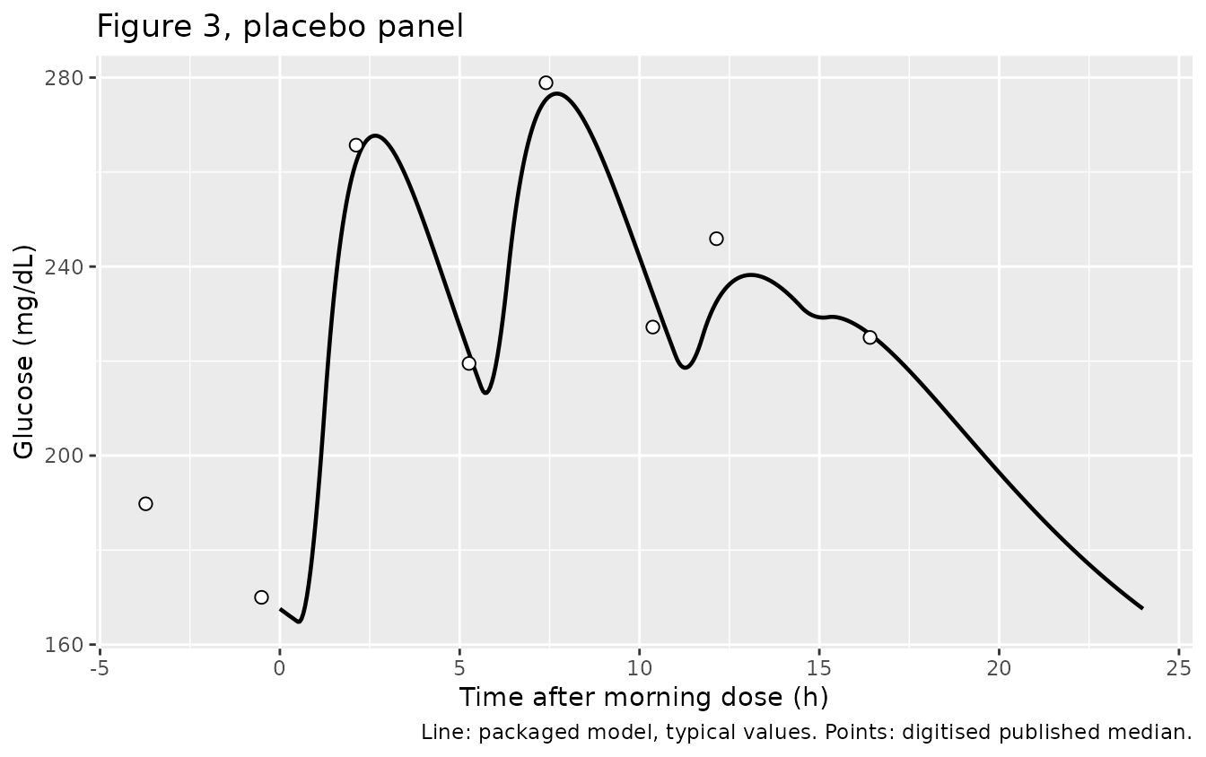
Replicating Figures 2 and 4 (GLP-1 and insulin)
Neither of these was used to derive V_glc or the
S5 prefix, so they are independent checks. Landmark values
were read off the published placebo panels by eye and carry roughly +/-
10% reading error, so the comparison is reported as an
order-of-magnitude and shape check.
fig24 <- tibble::tribble(
  ~endpoint,          ~trel, ~published,
  "GLP-1 (pmol/L)",   -0.51,  2.7,
  "GLP-1 (pmol/L)",    2.12,  5.8,
  "GLP-1 (pmol/L)",    7.40,  5.6,
  "GLP-1 (pmol/L)",   12.14,  5.5,
  "Insulin (mIU/L)",  -0.51, 22.0,
  "Insulin (mIU/L)",   2.12, 50.0,
  "Insulin (mIU/L)",   7.40, 57.0,
  "Insulin (mIU/L)",  12.14, 45.0
) |>
  dplyr::mutate(
    simulated = ifelse(
      endpoint == "GLP-1 (pmol/L)",
      approx(pb$trel, pb$Cglp, xout = trel, rule = 2)$y,
      approx(pb$trel, pb$Cins, xout = trel, rule = 2)$y
    ),
    ratio = simulated / published
  )

fig24 |>
  dplyr::mutate(dplyr::across(c(published, simulated, ratio), \(x) round(x, 2))) |>
  dplyr::rename(
    "Endpoint"                    = endpoint,
    "Time after morning dose (h)" = trel,
    "Published median (read)"     = published,
    "Simulated"                   = simulated,
    "Simulated / published"       = ratio
  ) |>
knitr::kable(caption = "Placebo GLP-1 (Figure 2) and insulin (Figure 4) landmarks.")| Endpoint | Time after morning dose (h) | Published median (read) | Simulated | Simulated / published |
|---|---|---|---|---|
| GLP-1 (pmol/L) | -0.51 | 2.7 | 2.38 | 0.88 |
| GLP-1 (pmol/L) | 2.12 | 5.8 | 4.45 | 0.77 |
| GLP-1 (pmol/L) | 7.40 | 5.6 | 4.73 | 0.85 |
| GLP-1 (pmol/L) | 12.14 | 5.5 | 6.20 | 1.13 |
| Insulin (mIU/L) | -0.51 | 22.0 | 16.37 | 0.74 |
| Insulin (mIU/L) | 2.12 | 50.0 | 37.32 | 0.75 |
| Insulin (mIU/L) | 7.40 | 57.0 | 40.95 | 0.72 |
| Insulin (mIU/L) | 12.14 | 45.0 | 33.12 | 0.74 |
# Deterministic, but compared against eye-read landmarks: assert the right
# order of magnitude and no systematic inversion, not agreement to a few
# percent. A mis-transcribed baseline, rate constant or unit moves these by
# factors of 3 or more and still breaks the bound.
base_glp <- fig24$simulated[fig24$endpoint == "GLP-1 (pmol/L)"  & fig24$trel == -0.51]
base_ins <- fig24$simulated[fig24$endpoint == "Insulin (mIU/L)" & fig24$trel == -0.51]
stopifnot(
  # Guard the scalar lookups so an empty match fails loudly instead of making
  # the baseline assertions below vacuously true.
  length(base_glp) == 1L, length(base_ins) == 1L,
  nrow(fig24) == 8L, all(is.finite(fig24$ratio)),
  all(fig24$ratio > 0.45), all(fig24$ratio < 2.2),
  # baselines are the cleanly determined part and must be close
  abs(base_glp - 2.7) < 1.0,
  abs(base_ins - 22.0) < 9
)
# Stochastic VPC across all four arms, matching the published figure style.
# Cohort size is well under the 200-per-arm cap.
rxode2::rxSetSeed(20260903)
n_per_arm <- 150L
vpc_ev <- dplyr::bind_rows(lapply(seq_along(ARMS), function(i) {
  x <- as.data.frame(build_arm(ARMS[[i]], 1L))
  x$arm <- names(ARMS)[i]
  x$id <- NULL
  x
}))

vpc <- dplyr::bind_rows(lapply(names(ARMS), function(a) {
  e <- dplyr::filter(vpc_ev, arm == a) |> dplyr::select(-arm)
  s <- rxode2::rxSolve(mod, events = e, nSub = n_per_arm,
                       returnType = "data.frame", useLinCmt = FALSE)
  # rxSolve names the subject column `sim.id` when the cohort is generated by
  # nSub from a single-subject event table, and `id` otherwise.
  s$id <- if (!is.null(s$id)) s$id else s$sim.id
  stopifnot(!is.null(s$id), dplyr::n_distinct(s$id) == n_per_arm)
  s$arm <- a
  s
})) |>
  dplyr::mutate(trel = time - 24 * (N_DAY - 1L),
                arm = factor(arm, levels = names(ARMS)))
#> ℹ parameter labels from comments will be replaced by 'label()'

vpc_fail <- 100 * mean(is.na(vpc$Cglc))

vpc |>
  dplyr::group_by(arm, trel) |>
  dplyr::summarise(
    Q10 = quantile(Cglc, 0.10, na.rm = TRUE),
    Q50 = quantile(Cglc, 0.50, na.rm = TRUE),
    Q90 = quantile(Cglc, 0.90, na.rm = TRUE),
    .groups = "drop"
  ) |>
  ggplot(aes(trel, Q50)) +
  geom_ribbon(aes(ymin = Q10, ymax = Q90), alpha = 0.2) +
  geom_line(linewidth = 0.7) +
  facet_wrap(~arm) +
  coord_cartesian(ylim = c(0, 500)) +
  labs(x = "Time after morning dose (h)", y = "Glucose (mg/dL)",
       title = "Figure 3 style VPC: median and 80% prediction interval",
       caption = "Replicates the layout of Figure 3 of Landersdorfer 2012.")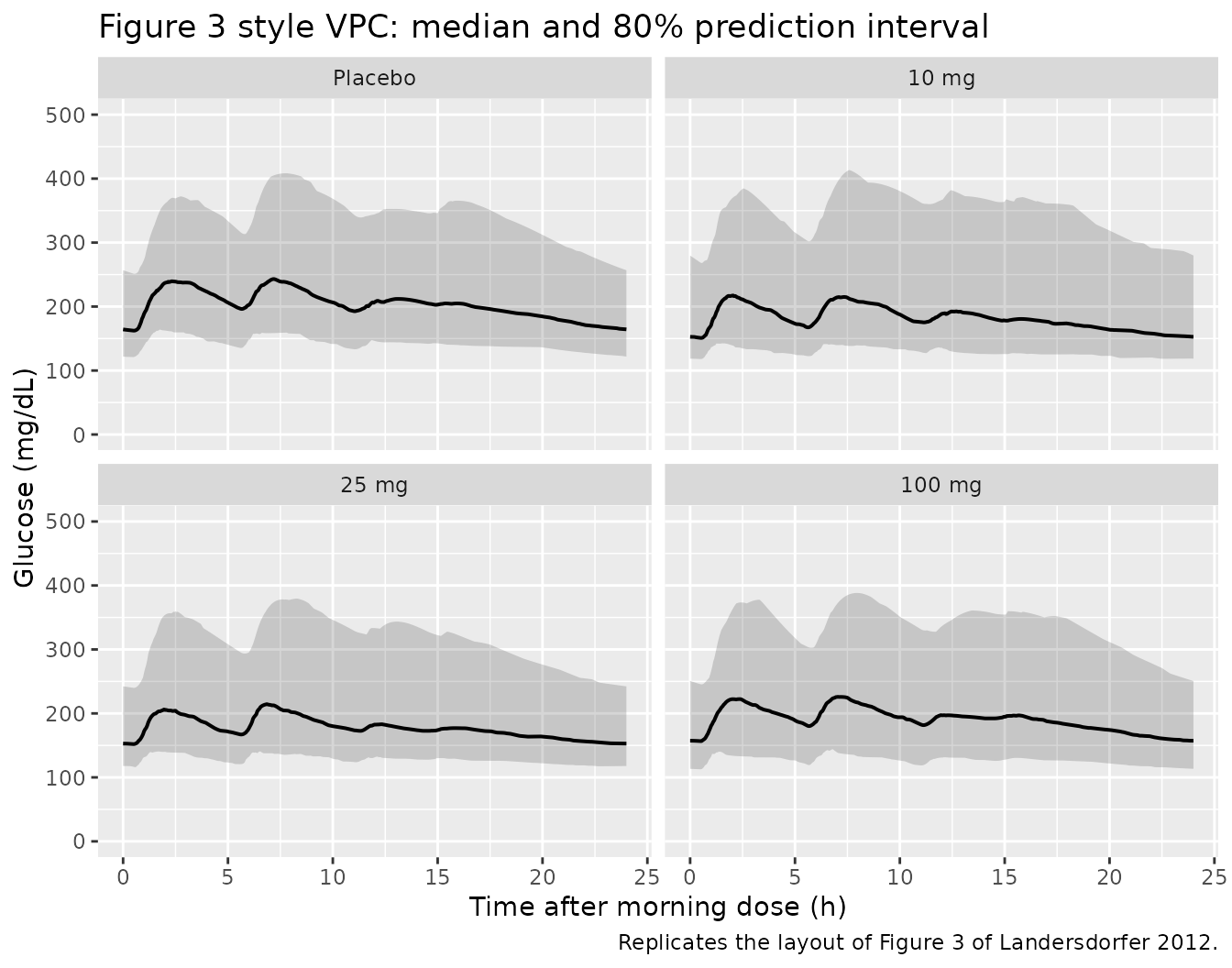
Unsolvable fraction for this cohort: 0.0% of simulated glucose
records. The published between-subject variability is very large on
several PD parameters (188% on S2, 150% on S5,
135% on S3), so extreme log-normal draws can put the
glucose-insulin feedback loop into a numerically stiff regime; the paper
reports the same structure without noting how S-ADAPT handled it. Which
draws land there depends on the rxode2 build, so the fraction is
reported rather than asserted and the percentiles below use
na.rm.
Replicating Figure 7 (model subparts)
Figure 7 plots four internal quantities directly, with published axis
ranges. None of these was used to derive V_glc or the
S5 prefix.
fig7 <- sim |>
  dplyr::mutate(
    st_ins    = (0.584 / 1000) * (1 + 1.90 * (Cglp - 1.68)),
    st_glc    = 0.0185 * (1 + 0.0701 * (Cglp - 1.68)),
    ins_secr  = 9.75 * 14.0 * (1 + st_glc * (Cglc - 133)),
    glp_elim  = (DPP4 / 2.80) * 0.641
  )

fig7 |>
  dplyr::select(trel, arm, `A: GLP-1 elimination by DPP-4 (1/h)` = glp_elim,
                `B: ST_ins (L/mIU)` = st_ins, `C: ST_glc (dL/mg)` = st_glc,
                `D: insulin secretion (mIU/L/h)` = ins_secr) |>
  tidyr::pivot_longer(-c(trel, arm), names_to = "panel", values_to = "value") |>
  ggplot(aes(trel, value, colour = arm)) +
  geom_line(linewidth = 0.6) +
  facet_wrap(~panel, scales = "free_y") +
  labs(x = "Time after morning dose (h)", y = NULL, colour = NULL,
       title = "Figure 7 panels A-D",
       caption = "Replicates Figure 7 of Landersdorfer 2012.")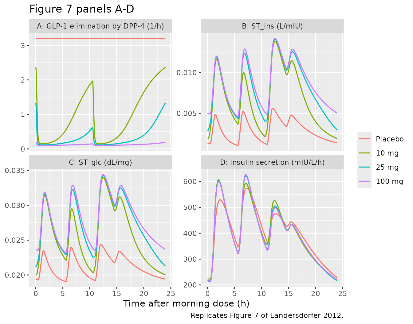
pb7 <- dplyr::filter(fig7, arm == "Placebo")
hi7 <- dplyr::filter(fig7, arm == "100 mg")

fig7_tab <- tibble::tribble(
  ~quantity,                                   ~published,                            ~simulated,
  "7A placebo GLP-1 elimination by DPP-4 (1/h), constant",
    "3.0 (flat line)",                         sprintf("%.2f", 5.0 * 0.641),
  "7A 100 mg GLP-1 elimination by DPP-4 (1/h), range",
    "about 0.05 to 0.25",                      sprintf("%.2f to %.2f", min(hi7$glp_elim), max(hi7$glp_elim)),
  "7B ST_ins (L/mIU), placebo fasting value",
    "about 0.001 (axis 0 to 0.009)",           sprintf("%.5f", min(pb7$st_ins)),
  "7C ST_glc (dL/mg), placebo fasting value",
    "about 0.019 (axis 0.015 to 0.029)",       sprintf("%.4f", min(pb7$st_glc)),
  "7D insulin secretion (mIU/L/h), placebo fasting value",
    "about 180 (axis 150 to 450)",             sprintf("%.0f", min(pb7$ins_secr)),
  "7D insulin secretion (mIU/L/h), placebo peak",
    "about 360",                               sprintf("%.0f", max(pb7$ins_secr))
)

fig7_tab |>
  dplyr::rename("Quantity" = quantity, "Figure 7" = published, "Simulated" = simulated) |>
knitr::kable(caption = "Figure 7 model subparts vs the packaged model (typical values).")| Quantity | Figure 7 | Simulated |
|---|---|---|
| 7A placebo GLP-1 elimination by DPP-4 (1/h), constant | 3.0 (flat line) | 3.21 |
| 7A 100 mg GLP-1 elimination by DPP-4 (1/h), range | about 0.05 to 0.25 | 0.10 to 0.19 |
| 7B ST_ins (L/mIU), placebo fasting value | about 0.001 (axis 0 to 0.009) | 0.00105 |
| 7C ST_glc (dL/mg), placebo fasting value | about 0.019 (axis 0.015 to 0.029) | 0.0190 |
| 7D insulin secretion (mIU/L/h), placebo fasting value | about 180 (axis 150 to 450) | 220 |
| 7D insulin secretion (mIU/L/h), placebo peak | about 360 | 574 |
# All deterministic. The fasting values are the cleanly determined part of each
# panel and are asserted tightly against the published axes; the postprandial
# peaks are amplified by the glucose excursion and are recorded as a deviation
# rather than gated (see Assumptions and deviations).
stopifnot(
  abs(5.0 * 0.641 - 3.0) < 0.3,                        # 7A placebo plateau
  max(hi7$glp_elim) < 0.35,                            # 7A 100 mg stays low
  min(pb7$st_ins) > 5e-4, min(pb7$st_ins) < 1.5e-3,    # 7B fasting sits on the axis
  max(pb7$st_ins) < 0.009,                             # 7B stays within the published axis
  min(pb7$st_glc) > 0.018, min(pb7$st_glc) < 0.022,    # 7C fasting
  max(pb7$st_glc) < 0.029,                             # 7C within the published axis
  min(pb7$ins_secr) > 150, min(pb7$ins_secr) < 260     # 7D fasting
)
Published quantitative claims
th <- function(nm) exp(ui$theta[[nm]])

claims <- tibble::tribble(
  ~claim, ~published, ~reproduced,
  "S2 implies a 35% rise in insulin secretion per 5 pmol/L rise in GLP-1 (Discussion, p. 385)",
    35,   100 * ((1 + th("ls2") * 5) - 1),
  "Complete DPP-4 inhibition raises the active GLP-1 half-life about 2.5-fold (Results, p. 377)",
    2.5,  (th("lkout_glp_lin") + th("lrmaxc") * th("lcf2")) / th("lkout_glp_lin"),
  "Half-life of vildagliptin dissociation from DPP-4 = 1.1 h (companion Abstract)",
    1.1,  log(2) / th("lkoff"),
  "Half-life of vildagliptin hydrolysis by DPP-4 = 6.3 h (companion Abstract)",
    6.3,  log(2) / th("lkdeg"),
  "Endogenous glucose production is physiological (mg/kg/min, 91 kg) -- consistency check on the back-solved V_glc",
    2.0,  th("lbl_glc") * th("lkout_glc") * th("lv_glc") / 60 / 91
) |>
  dplyr::mutate(pct_diff = 100 * (reproduced - published) / published)

claims |>
  dplyr::mutate(dplyr::across(c(published, reproduced, pct_diff), \(x) round(x, 3))) |>
  dplyr::rename("Published claim" = claim, "Published" = published,
                "From the packaged model" = reproduced, "Difference (%)" = pct_diff) |>
knitr::kable(caption = "Quantitative claims in the source, recomputed from the packaged model.")| Published claim | Published | From the packaged model | Difference (%) |
|---|---|---|---|
| S2 implies a 35% rise in insulin secretion per 5 pmol/L rise in GLP-1 (Discussion, p. 385) | 35.0 | 35.050 | 0.143 |
| Complete DPP-4 inhibition raises the active GLP-1 half-life about 2.5-fold (Results, p. 377) | 2.5 | 2.548 | 1.932 |
| Half-life of vildagliptin dissociation from DPP-4 = 1.1 h (companion Abstract) | 1.1 | 1.133 | 2.963 |
| Half-life of vildagliptin hydrolysis by DPP-4 = 6.3 h (companion Abstract) | 6.3 | 6.301 | 0.021 |
| Endogenous glucose production is physiological (mg/kg/min, 91 kg) – consistency check on the back-solved V_glc | 2.0 | 2.034 | 1.699 |
# Deterministic algebra on the packaged thetas, so tight bounds are correct.
# The first four are exact restatements of published numbers; the fifth is a
# physiological plausibility band, not a published value.
stopifnot(
  abs(claims$reproduced[1] - 35)  < 0.5,   # 35.05% vs 35%
  abs(claims$reproduced[2] - 2.5) < 0.15,  # 2.548 vs "approximately 2.5"
  abs(claims$reproduced[3] - 1.1) < 0.1,   # 1.133 vs 1.1 h
  abs(claims$reproduced[4] - 6.3) < 0.1,   # 6.301 vs 6.3 h
  claims$reproduced[5] > 1.4, claims$reproduced[5] < 3.0
)
Direction and size of the vildagliptin effect
The paper summarises Figure 6 in words: GLP-1 AUC rises with vildagliptin exposure, glucose AUC falls, and insulin AUC is “similar among all treatments” (Results, p. 377). Those are reproduced here as day-5 AUC ratios against placebo.
auc_day <- sim |>
  dplyr::filter(trel >= 0, trel <= 24) |>
  dplyr::group_by(arm) |>
  dplyr::summarise(
    GLP1    = PKNCA::pk.calc.auc(Cglp, trel, interval = c(0, 24), method = "linear"),
    Glucose = PKNCA::pk.calc.auc(Cglc, trel, interval = c(0, 24), method = "linear"),
    Insulin = PKNCA::pk.calc.auc(Cins, trel, interval = c(0, 24), method = "linear"),
    .groups = "drop"
  )

ratios <- auc_day |>
  dplyr::mutate(dplyr::across(c(GLP1, Glucose, Insulin),
                              \(x) x / x[arm == "Placebo"])) |>
  dplyr::filter(arm != "Placebo")

ratios |>
  dplyr::mutate(dplyr::across(where(is.numeric), \(x) round(x, 3))) |>
  dplyr::rename("Arm" = arm, "GLP-1 AUC ratio" = GLP1,
                "Glucose AUC ratio" = Glucose, "Insulin AUC ratio" = Insulin) |>
knitr::kable(caption = "Day-5 AUC(0-24 h) ratio vs placebo (typical values). Figure 6 of the source shows individual ratios of about 1-3 for GLP-1, 0.6-1.3 for glucose and 0.6-2.1 for insulin.")| Arm | GLP-1 AUC ratio | Glucose AUC ratio | Insulin AUC ratio |
|---|---|---|---|
| 10 mg | 1.909 | 0.922 | 0.994 |
| 25 mg | 2.263 | 0.900 | 0.992 |
| 100 mg | 2.411 | 0.893 | 0.992 |
# Deterministic (zeroRe). Directions are the paper's own qualitative claims and
# the magnitudes are bounded by the observed spread of Figure 6.
stopifnot(
  all(ratios$GLP1 > 1),                                  # GLP-1 AUC rises
  ratios$GLP1[ratios$arm == "100 mg"] > ratios$GLP1[ratios$arm == "10 mg"],
  all(ratios$GLP1 < 3.5),                                # within the Figure 6 range
  all(ratios$Glucose < 1),                               # glucose AUC falls
  ratios$Glucose[ratios$arm == "100 mg"] < ratios$Glucose[ratios$arm == "10 mg"],
  all(ratios$Glucose > 0.55),
  all(abs(ratios$Insulin - 1) < 0.35)                    # insulin "similar among treatments"
)
PKNCA validation (vildagliptin)
Vildagliptin plasma concentration is the one endpoint with
conventional PK, so NCA is run on it over the day-5 morning dosing
interval (0 to 10.5 h). The source paper reports no NCA table; Figure 6
plots individual AUC_vildagliptin values spanning roughly
50-2500 ng/mL*h across the three dose levels, which is the available
published anchor.
sim_nca <- vpc |>
  dplyr::filter(arm != "Placebo", trel >= 0, trel <= 10.5) |>
  dplyr::filter(!is.na(Cc)) |>
  dplyr::transmute(id = paste(arm, id, sep = "-"), arm, time = trel, Cc)

# Guarantee a time-zero record per (arm, id).
sim_nca <- dplyr::bind_rows(
  sim_nca,
  sim_nca |> dplyr::distinct(id, arm) |> dplyr::mutate(time = 0, Cc = 0)
) |>
  dplyr::distinct(id, arm, time, .keep_all = TRUE) |>
  dplyr::arrange(arm, id, time)

conc_obj <- PKNCA::PKNCAconc(as.data.frame(sim_nca), Cc ~ time | arm + id)

dose_df <- vpc |>
  dplyr::filter(arm != "Placebo") |>
  dplyr::distinct(arm, id) |>
  dplyr::transmute(id = paste(arm, id, sep = "-"), arm, time = 0,
                   amt = as.numeric(ARMS[as.character(arm)]))

dose_obj <- PKNCA::PKNCAdose(as.data.frame(dose_df), amt ~ time | arm + id)

intervals <- data.frame(start = 0, end = 10.5,
                        cmax = TRUE, tmax = TRUE, auclast = TRUE)

nca_res <- PKNCA::pk.nca(PKNCA::PKNCAdata(conc_obj, dose_obj, intervals = intervals))

nca_tab <- as.data.frame(nca_res) |>
  dplyr::filter(PPTESTCD %in% c("cmax", "tmax", "auclast")) |>
  dplyr::group_by(arm, PPTESTCD) |>
  dplyr::summarise(median = stats::median(PPORRES, na.rm = TRUE), .groups = "drop") |>
  tidyr::pivot_wider(names_from = PPTESTCD, values_from = median)

nca_tab |>
  dplyr::mutate(dplyr::across(where(is.numeric), \(x) round(x, 2))) |>
  dplyr::rename("Arm" = arm, "Cmax (ng/mL)" = cmax, "Tmax (h)" = tmax,
                "AUC0-10.5h (ng*h/mL)" = auclast) |>
knitr::kable(caption = "Median simulated steady-state NCA for vildagliptin over the morning dosing interval of day 5.")| Arm | AUC0-10.5h (ng*h/mL) | Cmax (ng/mL) | Tmax (h) |
|---|---|---|---|
| 10 mg | 127.34 | 39.97 | 1.3 |
| 25 mg | 368.38 | 103.97 | 1.3 |
| 100 mg | 1732.65 | 413.34 | 1.5 |
auc <- setNames(nca_tab$auclast, as.character(nca_tab$arm))
stopifnot(
  # Cohort medians, so bound loosely and on quantities a transcription error
  # would move by a large factor.
  all(auc > 20), all(auc < 4000),                 # inside the Figure 6 x-axis span
  auc[["100 mg"]] > auc[["25 mg"]], auc[["25 mg"]] > auc[["10 mg"]],
  # TMDD makes exposure MORE than dose proportional: saturable binding to a
  # finite DPP-4 pool means a smaller fraction of a large dose is bound.
  auc[["100 mg"]] / auc[["10 mg"]] > 10,
  all(nca_tab$tmax > 0), all(nca_tab$tmax < 6)
)
Exposure is more than dose proportional across the 10-fold dose range, which is the companion paper’s headline PK finding: “Due to limited amounts of DPP-4, vildagliptin concentrations increased more than proportionally with dose.”
Assumptions and deviations
-
V_glcis not published. Back-solved from the Figure 3 placebo median at 250 dL; sensitivity across the unreported meal timings and food-intake durations is 246-255 dL. The Figure 3 comparison above is therefore partly circular; Figures 2, 4, 6 and 7 are not. A maintainer ruling on 2026-09-02 chose the back-solve over author correspondence. -
S5is applied as 0.584 mL/mIU, not the printed 0.584 L/mIU. Established from Figure 7B’s own axis, which plotsST_insover 0 to 0.009 L/mIU and equalsS5at baseline GLP-1. The printed value is kept verbatim inini()and converted on one commented line inmodel(). -
S1is used in g^-1 per Table 1, not mg^-1 per the body text, so gut amounts are carried in grams. -
R_maxPis encoded as 13000 nmol (13 umol), not the companion table’s printed “13.0 mmol”; established from that paper’s own “>2000-fold” tissue:plasma statement. -
Meal timetable. Breakfast at 0.5 h and dinner at
11.0 h come from the stated design (30 min after each dose, evening dose
at 10.5 h). Lunch (5.6 h) and the snack (14.5 h) are read from the
meal-driven excursions in Figures 2, 3, 4 and 7.
tk0, “the actual recorded duration of food intake”, is never reported and is assumed to be 45 min. - Between-subject variability is diagonal only. Both papers state that a full variance-covariance matrix was estimated for the PK and (separately) the PD parameters, but only the diagonal is published as BSV (%). Off-diagonals are omitted. Between-occasion variability was not included by the authors either.
- Steady state is approached in 5 simulated days, not 28. Day-4 to day-5 glucose differs by less than 1% at matched clock times.
-
Known deviation, not gated: the postprandial peaks of the
Figure 7D insulin-secretion panel overshoot. The packaged
model’s placebo insulin secretion peaks near 570 mIU/L/h where Figure 7D
shows about 360, because the typical-value glucose excursion is somewhat
sharper than the paper’s. The fasting values of all four Figure 7 panels
agree, and Figure 3’s glucose median agrees to within a few percent, so
the discrepancy is in the peak shape rather than in the parameter scale.
It most plausibly reflects the unreported
tk0and meal times. This is recorded rather than tuned away. -
Some stochastic draws may not be solvable. The
published BSV reaches 188% on
S2and 150% onS5; extreme log-normal draws drive the glucose-insulin feedback into a stiff regime. Which subjects are drawn is not reproducible across rxode2 builds, so the VPC above measures and reports the affected fraction (0% for the packaged seed and cohort size on the build used here) and usesna.rmpercentiles rather than asserting on it. - Original observed data are not publicly available; every figure here is a simulation from the packaged model compared against digitised or transcribed published summaries.