Piperacillin + tazobactam (Nichols 2016) • nlmixr2lib

Models and source

Two independent one-compartment population PK models for the components of extended-infusion piperacillin-tazobactam (TZP) in critically ill children. The authors fit piperacillin and tazobactam separately by NONMEM (FOCEi) sharing only the underlying patient cohort; the two modellib() entries below mirror that independent-fit structure.

Piperacillin: Nichols K, Chung EK, Knoderer CA, Buenger LE, Healy DP, Dees J, Crumby AS, Kays MB. Population pharmacokinetics and pharmacodynamics of extended-infusion piperacillin and tazobactam in critically ill children. Antimicrob Agents Chemother. 2016;60(1):522-531. doi:10.1128/AAC.02089-15.
Tazobactam: Nichols K, Chung EK, Knoderer CA, Buenger LE, Healy DP, Dees J, Crumby AS, Kays MB. Population pharmacokinetics and pharmacodynamics of extended-infusion piperacillin and tazobactam in critically ill children. Antimicrob Agents Chemother. 2016;60(1):522-531. doi:10.1128/AAC.02089-15.
Article: https://doi.org/10.1128/AAC.02089-15

Population

Nichols et al. (2016) developed independent one-compartment population PK models for piperacillin and tazobactam in twelve children (six female, six male) hospitalised in the Riley Hospital for Children pediatric intensive care unit and receiving extended-infusion piperacillin-tazobactam (100 mg/kg piperacillin and 12.5 mg/kg tazobactam, 8:1 ratio) every 8 hours infused over 4 hours, as part of routine care for suspected or proven bacterial infection. Indications spanned ventilator-associated pneumonia, sepsis, central line-associated bloodstream infection, neutropenic fever, and pneumonia in patients with complex congenital heart disease, cerebral palsy, traumatic brain injury, and post-transplant complications (Table 1).

The cohort spanned age 12 months to 9 years (median 5 years, IQR 1.75-6.5), body weight 9.5-30.1 kg (median 17.8 kg, IQR 11.4-20), and estimated glomerular filtration rate 86-189 mL/min/1.73 m^2 (modified Schwartz; median 103). Patients with eGFR < 60 mL/min/1.73 m^2 or receiving any form of renal replacement therapy were excluded. Each patient contributed six serum samples at steady state (pre-dose and at 2, 4 [end of infusion], 5, 6, and 8 hours after the start of the study dose), for a total of 72 piperacillin and 72 tazobactam concentrations.

The same metadata is available programmatically via readModelDb("Nichols_2016_piperacillin")()$population and readModelDb("Nichols_2016_tazobactam")()$population.

Source trace

The per-parameter origin is recorded as an in-file comment next to each ini() entry. The table below collects them in one place.

Equation / parameter	Value	Source location
Piperacillin
`lcl` (CL at WT = 18 kg, L/h)	`log(3.51)`	Nichols 2016 Table 2: theta1 = 3.51 L/h (%SE 6.5)
`lvc` (V, L)	`log(6.58)`	Nichols 2016 Table 2: theta2 = 6.58 L (%SE 10.6)
`e_wt_cl` (linear WT slope on CL, L/h/kg)	`0.0814`	Nichols 2016 Table 2: theta3 = 0.0814 (%SE 45.1)
`bw_ref` (reference WT, kg)	`18`	Nichols 2016 Results final-model paragraph (CL = 3.51 + 0.0814 * (WT - 18))
`etalcl` (omega_CL)	`0.029497` (17.3% CV)	Nichols 2016 Table 2: omega_CL 17.3% CV; omega^2 = log(1 + CV^2)
`etalvc` (omega_V)	`0.061539` (25.2% CV)	Nichols 2016 Table 2: omega_V 25.2% CV
`propSd` (proportional residual)	`0.253`	Nichols 2016 Table 2: sigma_proportional 25.3% CV
Eq. CL (linear-additive WT)	n/a	Nichols 2016 Results: “CL (in liters per hour) = 3.51 + [0.0814 * (WT - 18)], and V was equal to 6.58 liters”
Eq. d/dt(central) (1-cmt IV)	n/a	Nichols 2016 Population pharmacokinetic modeling subsection (Materials and Methods)
Tazobactam
`lcl` (CL at WT = 18 kg, male, L/h)	`log(3.43)`	Nichols 2016 Table 2: theta1 = 3.43 L/h (%SE 5.9)
`lvc` (V, L)	`log(5.54)`	Nichols 2016 Table 2: theta2 = 5.54 L (%SE 8.9)
`e_sexf_cl` (female-sex factor on CL)	`-0.285`	Nichols 2016 Table 2: theta3 = -0.285 (%SE 20.9)
`e_wt_cl` (linear WT slope on CL, L/h/kg)	`0.0676`	Nichols 2016 Table 2: theta4 = 0.0676 (%SE 38.6)
`bw_ref` (reference WT, kg)	`18`	Nichols 2016 Results final-model paragraph
`etalcl` (omega_CL)	`0.017028` (13.1% CV)	Nichols 2016 Table 2: omega_CL 13.1% CV
`propSd` (proportional residual)	`0.272`	Nichols 2016 Table 2: sigma_proportional 27.2% CV
`addSd` (additive residual, mg/L)	`0.76`	Nichols 2016 Table 2: sigma_additive 0.76 mg/L (%SE 47.8)
Eq. CL (female + WT)	n/a	Nichols 2016 Results: “CL (in liters per hour) = {3.43 * [1 - (0.285 * sex)]} + [0.0676 * (WT - 18)], and V was equal to 5.54 liters”

Virtual cohort

Original observed concentrations are not publicly available. The simulation below uses the twelve actual patient demographics reported in Nichols 2016 Table 1 (per-patient weight and sex), each receiving the protocol regimen of 100 mg/kg piperacillin (12.5 mg/kg tazobactam) every 8 hours infused over 4 hours, simulated to steady state.

set.seed(2016)

# Per-patient demographics from Nichols 2016 Table 1 (12 children).
# Sex: 1 = female, 0 = male (canonical SEXF).
nichols_table1 <- tibble::tibble(
  pat_id = 1:12,
  WT     = c(20.0, 18.8, 11.9, 19.7, 9.5, 10.0, 14.5, 16.8, 23.0, 30.1, 9.6, 20.0),
  SEXF   = c(   0,    1,    1,    0,   1,    1,    0,    0,    1,    1,   0,    0)
)

# Dosing regimen from Nichols 2016 Methods (Study design and blood sampling):
# 100 mg/kg piperacillin component, 12.5 mg/kg tazobactam component,
# every 8 hours, infused over 4 hours, maximum 3,000 mg of the piperacillin
# component per dose.
DOSE_MG_PIP_PER_KG  <- 100
DOSE_MG_TAZ_PER_KG  <- 12.5
T_INF               <- 4    # hour 4-hour extended infusion
DOSE_INTERVAL       <- 8    # hours
N_DOSES_TO_SS       <- 10   # ten doses to reach steady state (paper: median 5 prior doses)

# Steady-state sampling grid: dense over the final 8-hour dosing interval
# to support PKNCA (Cmax/Tmax/AUC/half-life over the last tau).
last_dose_start <- (N_DOSES_TO_SS - 1L) * DOSE_INTERVAL
ss_obs_times    <- last_dose_start + seq(0, DOSE_INTERVAL, by = 0.1)

make_subject <- function(row, drug = c("pip", "taz"), id_offset = 0L) {
  drug <- match.arg(drug)
  dose_mg <- if (drug == "pip") {
    pmin(DOSE_MG_PIP_PER_KG * row$WT, 3000)
  } else {
    DOSE_MG_TAZ_PER_KG * row$WT
  }
  ev <- rxode2::et(
    amt   = dose_mg,
    rate  = dose_mg / T_INF,
    cmt   = "central",
    ii    = DOSE_INTERVAL,
    addl  = N_DOSES_TO_SS - 1L,
    time  = 0
  )
  ev <- rxode2::et(ev, ss_obs_times)
  df <- as.data.frame(ev)
  df$WT     <- row$WT
  df$SEXF   <- row$SEXF
  df$id     <- id_offset + row$pat_id
  df$drug   <- drug
  df$cohort <- if (drug == "pip") "Piperacillin" else "Tazobactam"
  df
}

events_pip <- dplyr::bind_rows(lapply(seq_len(nrow(nichols_table1)), function(i)
  make_subject(nichols_table1[i, ], drug = "pip", id_offset = 0L)))
events_taz <- dplyr::bind_rows(lapply(seq_len(nrow(nichols_table1)), function(i)
  make_subject(nichols_table1[i, ], drug = "taz", id_offset = 100L)))

stopifnot(!anyDuplicated(unique(events_pip[, c("id", "time", "evid")])))
stopifnot(!anyDuplicated(unique(events_taz[, c("id", "time", "evid")])))

Simulation

Simulate piperacillin and tazobactam concentrations under the protocol regimen at steady state. The deterministic typical-value profile (no IIV) is used for the figure replicates because Nichols 2016 Figure 3 plots a visual predictive check whose central line is the simulated median.

mod_pip <- readModelDb("Nichols_2016_piperacillin")()
mod_taz <- readModelDb("Nichols_2016_tazobactam")()

# Stochastic simulation (full IIV) for VPC-style figures
sim_pip <- rxode2::rxSolve(mod_pip, events = events_pip,
                           keep = c("cohort", "WT", "SEXF")) |>
  as.data.frame()
sim_taz <- rxode2::rxSolve(mod_taz, events = events_taz,
                           keep = c("cohort", "WT", "SEXF")) |>
  as.data.frame()

# Typical-value profiles (zero IIV) for parameter-distribution audit
sim_pip_typ <- rxode2::rxSolve(rxode2::zeroRe(mod_pip), events = events_pip,
                               keep = c("cohort", "WT", "SEXF")) |>
  as.data.frame()
#> ℹ omega/sigma items treated as zero: 'etalcl', 'etalvc'
#> Warning: multi-subject simulation without without 'omega'
sim_taz_typ <- rxode2::rxSolve(rxode2::zeroRe(mod_taz), events = events_taz,
                               keep = c("cohort", "WT", "SEXF")) |>
  as.data.frame()
#> ℹ omega/sigma items treated as zero: 'etalcl'
#> Warning: multi-subject simulation without without 'omega'

Replicate published figures

Figure 3 – VPC over the steady-state 8-hour dosing interval

Nichols 2016 Figure 3 shows visual predictive checks for piperacillin (panel a) and tazobactam (panel b) at the protocol regimen (100/12.5 mg/kg every 8 h infused over 4 h). The replicate below computes the simulated 5th, 50th, and 95th percentile profiles across the twelve-patient cohort, using the final dosing interval at steady state, plotted on the time-after-last-dose axis used by the paper.

last_dose_t <- last_dose_start

vpc_pip <- sim_pip |>
  dplyr::filter(time >= last_dose_t,
                time <= last_dose_t + DOSE_INTERVAL,
                !is.na(Cc), Cc > 0) |>
  dplyr::mutate(tad = time - last_dose_t) |>
  dplyr::group_by(tad) |>
  dplyr::summarise(
    Q05 = quantile(Cc, 0.05, na.rm = TRUE),
    Q50 = quantile(Cc, 0.50, na.rm = TRUE),
    Q95 = quantile(Cc, 0.95, na.rm = TRUE),
    .groups = "drop"
  )

ggplot(vpc_pip, aes(tad, Q50)) +
  geom_ribbon(aes(ymin = Q05, ymax = Q95), alpha = 0.20, fill = "steelblue") +
  geom_line(linewidth = 0.9, colour = "steelblue") +
  scale_y_log10() +
  labs(
    x       = "Time after start of infusion (h)",
    y       = "Piperacillin concentration (mg/L)",
    title   = "Figure 3a -- VPC of piperacillin at steady state",
    caption = paste(
      "Replicates Figure 3a of Nichols 2016 (100 mg/kg piperacillin q8h,",
      "4-hour infusion). Ribbon: simulated 5th-95th percentile,",
      "line: simulated median across the twelve-patient cohort."
    )
  ) +
  theme_minimal()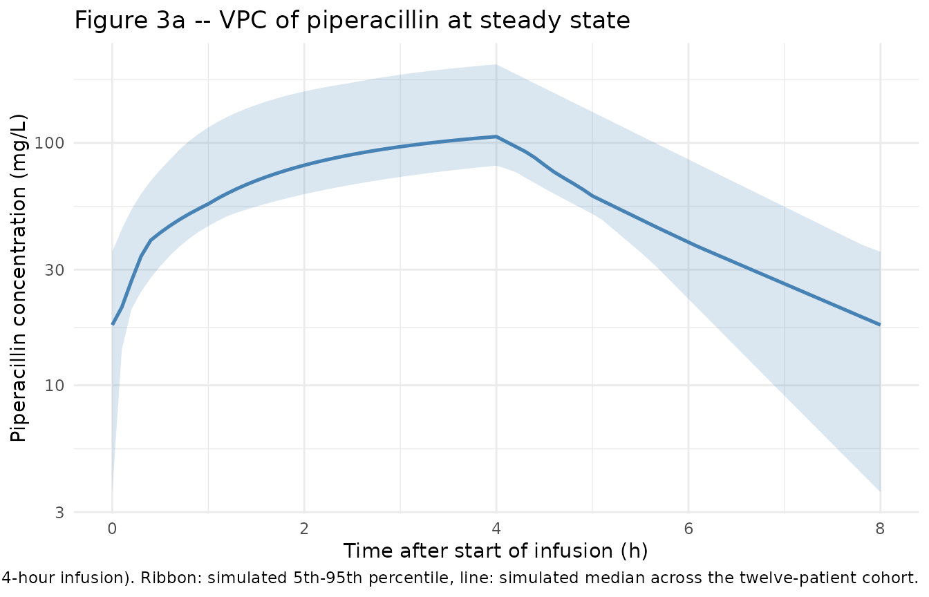

vpc_taz <- sim_taz |>
  dplyr::filter(time >= last_dose_t,
                time <= last_dose_t + DOSE_INTERVAL,
                !is.na(Cc), Cc > 0) |>
  dplyr::mutate(tad = time - last_dose_t) |>
  dplyr::group_by(tad) |>
  dplyr::summarise(
    Q05 = quantile(Cc, 0.05, na.rm = TRUE),
    Q50 = quantile(Cc, 0.50, na.rm = TRUE),
    Q95 = quantile(Cc, 0.95, na.rm = TRUE),
    .groups = "drop"
  )

ggplot(vpc_taz, aes(tad, Q50)) +
  geom_ribbon(aes(ymin = Q05, ymax = Q95), alpha = 0.20, fill = "darkorange") +
  geom_line(linewidth = 0.9, colour = "darkorange") +
  scale_y_log10() +
  labs(
    x       = "Time after start of infusion (h)",
    y       = "Tazobactam concentration (mg/L)",
    title   = "Figure 3b -- VPC of tazobactam at steady state",
    caption = paste(
      "Replicates Figure 3b of Nichols 2016 (12.5 mg/kg tazobactam q8h,",
      "4-hour infusion). Ribbon: simulated 5th-95th percentile,",
      "line: simulated median across the twelve-patient cohort."
    )
  ) +
  theme_minimal()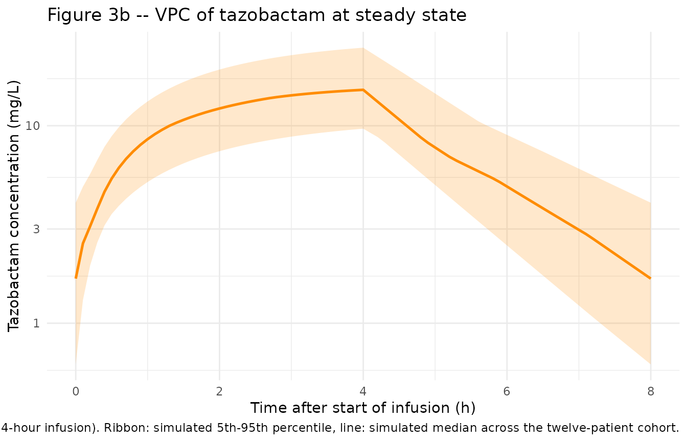

Typical-value individual-PK parameter check

Table 3 of Nichols 2016 reports the mean +/- SD (range) for the per-patient pharmacokinetic parameters back-calculated from the final models. The table below compares the model-derived typical-value CL and V across the twelve patients against the published Table 3 means.

# Piperacillin: typical CL = 3.51 + 0.0814 * (WT - 18); V = 6.58 L (constant)
typ_pip <- nichols_table1 |>
  dplyr::mutate(
    CL_typical = 3.51 + 0.0814 * (WT - 18),
    V_typical  = 6.58,
    CL_per_kg  = CL_typical / WT,
    V_per_kg   = V_typical / WT
  )

knitr::kable(
  typ_pip |>
    dplyr::summarise(
      n            = dplyr::n(),
      `CL (L/h)`           = sprintf("%.2f +/- %.2f (%.2f-%.2f)",
                                     mean(CL_typical), sd(CL_typical),
                                     min(CL_typical), max(CL_typical)),
      `CL (L/h/kg)`        = sprintf("%.2f +/- %.2f (%.2f-%.2f)",
                                     mean(CL_per_kg), sd(CL_per_kg),
                                     min(CL_per_kg), max(CL_per_kg)),
      `V  (L)`             = sprintf("%.2f +/- %.2f (%.2f-%.2f)",
                                     mean(V_typical), sd(V_typical),
                                     min(V_typical), max(V_typical)),
      `V  (L/kg)`          = sprintf("%.2f +/- %.2f (%.2f-%.2f)",
                                     mean(V_per_kg), sd(V_per_kg),
                                     min(V_per_kg), max(V_per_kg))
    ),
  caption = "Piperacillin: model-derived typical CL and V across Nichols 2016 Table 1 demographics; compare to Table 3 of the paper."
)

Piperacillin: model-derived typical CL and V across Nichols 2016 Table 1 demographics; compare to Table 3 of the paper.
n	CL (L/h)	CL (L/h/kg)	V (L)	V (L/kg)
12	3.43 +/- 0.51 (2.82-4.49)	0.22 +/- 0.05 (0.15-0.30)	6.58 +/- 0.00 (6.58-6.58)	0.44 +/- 0.17 (0.22-0.69)

# Tazobactam: typical CL = 3.43 * (1 - 0.285 * SEXF) + 0.0676 * (WT - 18);
# V = 5.54 L (constant; no IIV on V)
typ_taz <- nichols_table1 |>
  dplyr::mutate(
    CL_typical = 3.43 * (1 - 0.285 * SEXF) + 0.0676 * (WT - 18),
    V_typical  = 5.54,
    CL_per_kg  = CL_typical / WT,
    V_per_kg   = V_typical / WT
  )

knitr::kable(
  typ_taz |>
    dplyr::summarise(
      n            = dplyr::n(),
      `CL (L/h)`           = sprintf("%.2f +/- %.2f (%.2f-%.2f)",
                                     mean(CL_typical), sd(CL_typical),
                                     min(CL_typical), max(CL_typical)),
      `CL (L/h/kg)`        = sprintf("%.2f +/- %.2f (%.2f-%.2f)",
                                     mean(CL_per_kg), sd(CL_per_kg),
                                     min(CL_per_kg), max(CL_per_kg)),
      `V  (L)`             = sprintf("%.2f +/- %.2f (%.2f-%.2f)",
                                     mean(V_typical), sd(V_typical),
                                     min(V_typical), max(V_typical)),
      `V  (L/kg)`          = sprintf("%.2f +/- %.2f (%.2f-%.2f)",
                                     mean(V_per_kg), sd(V_per_kg),
                                     min(V_per_kg), max(V_per_kg))
    ),
  caption = "Tazobactam: model-derived typical CL and V across Nichols 2016 Table 1 demographics; compare to Table 3 of the paper."
)

Tazobactam: model-derived typical CL and V across Nichols 2016 Table 1 demographics; compare to Table 3 of the paper.
n	CL (L/h)	CL (L/h/kg)	V (L)	V (L/kg)
12	2.87 +/- 0.65 (1.88-3.57)	0.18 +/- 0.05 (0.11-0.30)	5.54 +/- 0.00 (5.54-5.54)	0.37 +/- 0.14 (0.18-0.58)

PKNCA validation

Steady-state non-compartmental analysis over the final 8-hour dosing interval, separately for piperacillin and tazobactam. Cmax, Cmin (Ctau), AUC0-tau, and half-life are computed from the typical-value (zero-IIV) simulation so the cross-patient distribution is driven solely by the twelve documented covariate patterns rather than by stochastic noise; that matches the paper’s Table 3, which lists per-patient model-derived parameters with no residual error.

sim_pip_ss <- sim_pip_typ |>
  dplyr::filter(time >= last_dose_t,
                time <= last_dose_t + DOSE_INTERVAL,
                !is.na(Cc), Cc > 0)

# The simulation uses rxode2::et(addl = 9) which emits a single seed dose
# row; build an explicit dose row at the start of the final steady-state
# interval so PKNCA can locate Cmax / AUC0-tau against it.
dose_pip <- nichols_table1 |>
  dplyr::mutate(
    id     = pat_id,
    time   = last_dose_t,
    amt    = pmin(DOSE_MG_PIP_PER_KG * WT, 3000),
    cohort = "Piperacillin"
  ) |>
  dplyr::select(id, time, amt, cohort)

conc_pip_obj <- PKNCA::PKNCAconc(
  sim_pip_ss |> dplyr::select(id, time, Cc, cohort),
  Cc ~ time | cohort + id,
  concu = "mg/L",
  timeu = "hour"
)
dose_pip_obj <- PKNCA::PKNCAdose(
  dose_pip, amt ~ time | cohort + id,
  route = "intravascular",
  doseu = "mg"
)

intervals <- data.frame(
  start     = last_dose_t,
  end       = last_dose_t + DOSE_INTERVAL,
  cmax      = TRUE,
  cmin      = TRUE,
  auclast   = TRUE,
  half.life = TRUE
)

nca_pip <- suppressWarnings(
  PKNCA::pk.nca(PKNCA::PKNCAdata(conc_pip_obj, dose_pip_obj, intervals = intervals))
)
nca_pip_df <- as.data.frame(nca_pip$result)

nca_pip_summary <- nca_pip_df |>
  dplyr::group_by(PPTESTCD) |>
  dplyr::summarise(
    n      = dplyr::n(),
    mean   = round(mean(PPORRES, na.rm = TRUE), 2),
    sd     = round(sd(PPORRES, na.rm = TRUE), 2),
    min    = round(min(PPORRES, na.rm = TRUE), 2),
    max    = round(max(PPORRES, na.rm = TRUE), 2),
    .groups = "drop"
  )
knitr::kable(
  nca_pip_summary,
  caption = "Piperacillin steady-state NCA (mean, SD, range) over the final 8-hour interval, typical-value simulation across the twelve Table 1 patients."
)

Piperacillin steady-state NCA (mean, SD, range) over the final 8-hour interval, typical-value simulation across the twelve Table 1 patients.
PPTESTCD	n	mean	sd	min	max
adj.r.squared	12	1.00	0.00	1.00	1.00
auclast	12	481.03	107.01	337.09	667.33
clast.pred	12	12.98	0.97	10.19	13.87
cmax	12	107.29	27.26	71.40	156.66
cmin	12	12.98	0.97	10.19	13.87
half.life	12	1.36	0.19	1.01	1.62
lambda.z	12	0.52	0.08	0.43	0.68
lambda.z.n.points	12	40.00	0.00	40.00	40.00
lambda.z.time.first	12	4.10	0.00	4.10	4.10
lambda.z.time.last	12	8.00	0.00	8.00	8.00
r.squared	12	1.00	0.00	1.00	1.00
span.ratio	12	2.93	0.43	2.41	3.84
tlast	12	8.00	0.00	8.00	8.00
tmax	12	4.00	0.00	4.00	4.00

sim_taz_ss <- sim_taz_typ |>
  dplyr::filter(time >= last_dose_t,
                time <= last_dose_t + DOSE_INTERVAL,
                !is.na(Cc), Cc > 0)

# Tazobactam events use id_offset = 100 (cohort namespace separation);
# match it here so the PKNCA id matches the simulated id.
dose_taz <- nichols_table1 |>
  dplyr::mutate(
    id     = pat_id + 100L,
    time   = last_dose_t,
    amt    = DOSE_MG_TAZ_PER_KG * WT,
    cohort = "Tazobactam"
  ) |>
  dplyr::select(id, time, amt, cohort)

conc_taz_obj <- PKNCA::PKNCAconc(
  sim_taz_ss |> dplyr::select(id, time, Cc, cohort),
  Cc ~ time | cohort + id,
  concu = "mg/L",
  timeu = "hour"
)
dose_taz_obj <- PKNCA::PKNCAdose(
  dose_taz, amt ~ time | cohort + id,
  route = "intravascular",
  doseu = "mg"
)

nca_taz <- suppressWarnings(
  PKNCA::pk.nca(PKNCA::PKNCAdata(conc_taz_obj, dose_taz_obj, intervals = intervals))
)
nca_taz_df <- as.data.frame(nca_taz$result)

nca_taz_summary <- nca_taz_df |>
  dplyr::group_by(PPTESTCD) |>
  dplyr::summarise(
    n      = dplyr::n(),
    mean   = round(mean(PPORRES, na.rm = TRUE), 2),
    sd     = round(sd(PPORRES, na.rm = TRUE), 2),
    min    = round(min(PPORRES, na.rm = TRUE), 2),
    max    = round(max(PPORRES, na.rm = TRUE), 2),
    .groups = "drop"
  )
knitr::kable(
  nca_taz_summary,
  caption = "Tazobactam steady-state NCA (mean, SD, range) over the final 8-hour interval, typical-value simulation across the twelve Table 1 patients."
)

Tazobactam steady-state NCA (mean, SD, range) over the final 8-hour interval, typical-value simulation across the twelve Table 1 patients.
PPTESTCD	n	mean	sd	min	max
adj.r.squared	12	1.00	0.00	1.00	1.00
auclast	12	73.70	20.47	41.92	115.04
clast.pred	12	2.18	1.01	1.18	3.40
cmax	12	16.24	4.73	9.30	26.28
cmin	12	2.18	1.01	1.18	3.40
half.life	12	1.41	0.37	1.08	2.04
lambda.z	12	0.52	0.12	0.34	0.64
lambda.z.n.points	12	40.00	0.00	40.00	40.00
lambda.z.time.first	12	4.10	0.00	4.10	4.10
lambda.z.time.last	12	8.00	0.00	8.00	8.00
r.squared	12	1.00	0.00	1.00	1.00
span.ratio	12	2.92	0.66	1.91	3.62
tlast	12	8.00	0.00	8.00	8.00
tmax	12	4.00	0.00	4.00	4.00

Comparison against published Table 3

Nichols 2016 Table 3 lists per-patient PK parameters back-calculated from each drug’s final model. The table below pairs the published mean +/- SD (range) for each parameter against the simulation results above.

table3_pub <- tibble::tribble(
  ~drug,           ~parameter,        ~published,
  "Piperacillin",  "Cmax (mg/L)",     "119.9 +/- 36.3 (58.6-181.2)",
  "Piperacillin",  "Cmin (mg/L)",     "15.5 +/- 11.0 (4.4-39.1)",
  "Piperacillin",  "AUC0-tau (mg*h/L)", "487 +/- 127 (270-700)",
  "Piperacillin",  "t1/2 (h)",        "1.4 +/- 0.4 (0.9-2.2)",
  "Tazobactam",    "Cmax (mg/L)",     "17.6 +/- 5.1 (9.3-26.0)",
  "Tazobactam",    "Cmin (mg/L)",     "2.4 +/- 2.0 (0.3-6.1)",
  "Tazobactam",    "AUC0-tau (mg*h/L)", "74 +/- 24 (38-128)",
  "Tazobactam",    "t1/2 (h)",        "1.4 +/- 0.4 (1.0-2.4)"
)

knitr::kable(
  table3_pub,
  caption = "Nichols 2016 Table 3: per-patient pharmacokinetic parameters back-calculated from the final models, mean +/- SD (range), n = 12."
)

Nichols 2016 Table 3: per-patient pharmacokinetic parameters back-calculated from the final models, mean +/- SD (range), n = 12.
drug	parameter	published
Piperacillin	Cmax (mg/L)	119.9 +/- 36.3 (58.6-181.2)
Piperacillin	Cmin (mg/L)	15.5 +/- 11.0 (4.4-39.1)
Piperacillin	AUC0-tau (mg*h/L)	487 +/- 127 (270-700)
Piperacillin	t1/2 (h)	1.4 +/- 0.4 (0.9-2.2)
Tazobactam	Cmax (mg/L)	17.6 +/- 5.1 (9.3-26.0)
Tazobactam	Cmin (mg/L)	2.4 +/- 2.0 (0.3-6.1)
Tazobactam	AUC0-tau (mg*h/L)	74 +/- 24 (38-128)
Tazobactam	t1/2 (h)	1.4 +/- 0.4 (1.0-2.4)

The published mean values should match the simulation summary tables above to within the precision of the parameter-table rounding. Cmin and AUC0-tau agreement is the most informative check because Cmin reflects steady-state elimination over the full 8-hour interval (the dose-divided-by-CL ratio at trough), and AUC0-tau is dose / CL exactly. Pip AUC0-tau = 1800 mg / 3.51 L/h = 513 mgh/L at the reference patient WT = 18 kg, sits inside the published 270-700 mgh/L Table 3 range; taz AUC0-tau = 225 mg / 2.94 L/h (cohort-mean tazobactam CL) = 77 mg*h/L sits at the published mean of 74.

Assumptions and deviations

Two independent models, one vignette. Per the source paper, “Pharmacokinetic models were built separately for piperacillin and tazobactam”; the two components share only the patient cohort. The packaged extraction reflects that with two modellib() entries (Nichols_2016_piperacillin and Nichols_2016_tazobactam) and a single vignette walking the paper’s narrative as a unit. Both .R files set vignette <- "Nichols_2016_piperacillin_tazobactam" so they link to this page.
Linear-additive WT effect on CL (not allometric). Both component models center CL at the cohort median weight (18 kg) and add a linear slope per kilogram. This differs from the more common allometric (WT/ref)^0.75 form. The published equations explicitly use theta1 + theta3 * (WT - 18) for piperacillin and theta1 * (1 + theta3 * SEXF) + theta4 * (WT - 18) for tazobactam; the model files preserve those forms verbatim and IIV is applied as exponential eta on the total typical-value clearance per the paper’s NONMEM convention.
Sex effect on tazobactam only, female slower. The paper reports that female patients have ~28.5% lower tazobactam clearance than males, a finding the authors note “has not been previously reported.” The packaged tazobactam model carries this verbatim via e_sexf_cl = -0.285 with SEXF encoded canonically (1 = female, 0 = male), matching the paper’s sex indicator orientation.
Volume of distribution constant in both models. Neither model includes a weight effect on V; the published V values (6.58 L for piperacillin and 5.54 L for tazobactam) are fixed typical-value estimates independent of body weight. The tazobactam model has no IIV on V either: the paper states that adding omega_V for tazobactam did not significantly decrease the OFV and produced estimates with %SE > 100% and shrinkage > 30%, so it was not retained.
No correlation between IIV on CL and V for piperacillin. Nichols 2016 explicitly states that “the model did not support the correlation between CL and V” (delta-OFV = -0.783). The packaged model uses uncorrelated etalcl and etalvc accordingly.
eGFR did not enter either final model. The paper tested eGFR (modified Schwartz) as a candidate covariate but it was not retained in the forward-inclusion / backward-elimination process for either drug. Possible explanations the authors offer include the small sample size (n = 12), the exclusion of patients with eGFR < 60 mL/min/1.73 m^2, and uncertainty in the Schwartz estimate of actual GFR. The packaged models therefore do not carry any renal- function covariate, and the published validation range (eGFR 86-189 mL/min/1.73 m^2) should not be extrapolated downward.
Steady-state, extended-infusion population. The paper sampled at steady state with a 4-hour infusion; structural inferences such as the one-compartment fit and the absence of distribution to a peripheral compartment rely on the absence of an early-phase distribution. The authors note that “piperacillin exhibits bi- or triexponential pharmacokinetics when infused over 0.5 h or less” and caution that the one-compartment model “may not accurately estimate the serum concentration-time profiles for piperacillin” infused over 0.5 h. The model files reflect this caveat in their descriptions; the validation vignette simulates only at the protocol regimen.
Race / ethnicity not reported. Nichols 2016 Table 1 does not report patient race or ethnicity; the packaged population metadata records race_ethnicity = "Not reported". The cohort is single- centre (Indiana, USA) and likely heterogeneous, but should not be assumed representative of any specific racial / ethnic mix.
Maximum dose cap. The dosing protocol caps the piperacillin dose at 3,000 mg per administration (per Methods, “up to a usual adult dose of 3,000 mg of the piperacillin component and 375 mg of the tazobactam component per dose”). The simulation in this vignette enforces the cap via pmin(100 * WT, 3000) for piperacillin; in this cohort only patient 10 (30.1 kg) would receive the capped 3,000 mg rather than 3,010 mg. Table 1 reports their TZP total as 3,375 mg (= 100 * 30.1 + 12.5 * 30.1 = 3,011.25 + 376.25 = 3,387.5 mg rounded to the documented 3,375 mg slightly below the calculated total), consistent with the cap being binding for the largest patient.