Model and source
- Citation: Chen Z, Taubert M, Chen C, Boland J, Dong Q, Bilal M, Dokos C, Wachall B, Wargenau M, Scheidel B, Wiesen MHJ, Schaeffeler E, Tremmel R, Schwab M, Fuhr U (2024). A Semi-Mechanistic Population Pharmacokinetic Model of Noscapine in Healthy Subjects Considering Hepatic First-Pass Extraction and CYP2C9 Genotypes. Drugs in R&D 24:187-199. doi:10.1007/s40268-024-00466-6.
- Description: Semi-mechanistic population PK model for oral noscapine in healthy adults (Chen 2024) with zero-order release into a four-compartment transit chain, an explicit liver compartment that carries the profound hepatic first-pass extraction (apparent clearance CL/F leaves the liver, not the plasma), and three-compartment systemic disposition. Liver plasma flow Qh (55 L/h) and liver volume Vh (1.5 L) are held fixed at physiologic values. Apparent clearance carries a CYP2C9 genotype-predicted-phenotype effect on three levels keyed to the CPIC activity score (extensive metabolizer reference 958 L/h; intermediate metabolizer with activity score 1.5, 531 L/h; poor and intermediate metabolizers with activity score 1.0, 343 L/h) plus a total-body-weight power term (exponent 1.34, 77.3 kg reference); inter-compartmental clearance to the first peripheral compartment carries an age power term (exponent 0.348, 29 year reference). Relative bioavailability of the reformulated test suspension is 82.8% of the reference suspension. Correlated inter-individual variability on absorption duration, CL/F, Vc/F and F1; inter-occasion variability on the transit rate and on Qp1/F across the two crossover periods; exponential residual error.
- Article: https://doi.org/10.1007/s40268-024-00466-6 (open access, CC BY-NC 4.0)
Noscapine is an opium-poppy alkaloid used as an antitussive, with ongoing interest in its anti-inflammatory and anti-tumour properties. It undergoes extensive hepatic first-pass metabolism – oral bioavailability is around 30% – and CYP2C9 is the dominant metabolising enzyme. Chen 2024 developed a semi-mechanistic population PK model from a two-period crossover bioequivalence study, using an explicit liver compartment to carry the first-pass extraction and resolving apparent clearance across three CYP2C9 genotype-predicted phenotype strata.
Structure
                                      Qh/Vh
Oral dose x F1 --Rate--> [t1]->[t2]->[t3]->[t4] --TR--> (Liver) <=======> (Plasma) <=> (Peripheral 1)
                         \___ n = 4 transit ___/            |          Qh/(Vc/F)   <=> (Peripheral 2)
                                                     (CL/F)/Vh
Two features distinguish this from a conventional oral three-compartment model:
-
The absorption chain empties into the liver, not into
plasma. Apparent clearance leaves from the liver compartment,
so every absorbed molecule is subject to hepatic extraction before it
can reach the sampling compartment. Adding the liver compartment
improved the fit by
dOFV = -562(Sect. 3.3.3). -
Absorption is zero-order into a four-compartment transit
chain. Zero-order release (duration
D1) described the input better than first-order, and four manually fixed transit compartments described the delayed gastric emptying better than a lag time or an estimated transit number (Sect. 3.3.1).
Liver plasma flow Qh (55 L/h) and liver volume
Vh (1.5 L) are held fixed at physiologic values. The
sensitivity analysis in Table S2 of the ESM showed that
CL/F, F1, the IIVs and the residual
variability were nearly unchanged across alternative liver settings,
which is why the simpler fixed-constant form was retained.
Population
The model was fitted to 1920 plasma noscapine concentrations from 48 healthy volunteers (30 men, 18 women; mean age 33 years, range 19–65; mean total body weight 77.3 kg, range 54.3–107; BMI 18.0–29.5 kg/m^2) enrolled at the Clinical Pharmacology Unit of the University Hospital of Cologne (Table 1). Each subject completed both periods of a randomised, two-period, two-stage crossover bioequivalence study comparing a reformulated noscapine oral suspension (InfectoPharm, test) against Nipaxon 5 mg/mL oral suspension (McNeil, reference), 50 mg single oral dose per period with a 6–14 day washout (DRKS00017760). Samples were drawn at baseline and 0.17, 0.33, 0.5, 0.67, 0.83, 1, 1.25, 1.5, 1.75, 2, 2.5, 3, 3.5, 4, 6, 9, 12, 16 and 24 h post-dose. Genome-wide principal-component analysis placed most subjects in European ancestry, with two clustering to South Asian / American and two to African populations (Fig. S1 of the ESM).
All 48 subjects were genotyped for CYP2C9, CYP2C19, CYP3A4, CYP3A5 and CYP2E1 (Table 2). Only CYP2C9 had a significant PK effect. Its three strata, keyed to the CPIC activity score (AS), are:
| CYP2C9 stratum | Genotypes | n (%) | CL/F |
|---|---|---|---|
| Extensive metabolizer (AS 2.0) |
*1/*1 (31), *1/*9 (1) |
32 (66.7) | 958 L/h |
| Intermediate metabolizer, AS 1.5 | *1/*2 |
10 (20.8) | 531 L/h |
| Poor & intermediate metabolizer, AS 1.0 |
*1/*3 (3), *2/*3 (2), *3/*3
(1) |
6 (12.5) | 343 L/h |
The AS-1.0 stratum deliberately pools poor metabolizers with the intermediate metabolizers that reach AS 1.0, “because of the limited sample size of homozygous carriers” (Sect. 3.1).
The same information is available programmatically via
readModelDb("Chen_2024_noscapine")()$population.
Source trace
Every ini() entry in
inst/modeldb/specificDrugs/Chen_2024_noscapine.R carries an
in-file comment naming its source location. They are collected here for
review.
| Equation / parameter | Value | Source location |
|---|---|---|
ld1 (absorption duration D1) |
0.0624 h | Table 4 (RSE 28.6%) |
lktr (transit rate TR) |
13.0 1/h | Table 4 (RSE 6.4%) |
lcl (CL/F, extensive metabolizer) |
958 L/h | Table 4 CL/F_EM (RSE 10.3%) |
e_cyp2c9im_as15_lcl |
log(531/958) = -0.5901 |
Table 4 CL/F_IM_1.5 = 531 L/h (RSE 23.0%) |
e_cyp2c9pmim_as10_lcl |
log(343/958) = -1.0271 |
Table 4 CL/F_PM_IM_1.0 = 343 L/h (RSE 24.8%) |
lvc (Vc/F) |
49.7 L | Table 4 (RSE 5.9%) |
lq (Qp1/F) |
18.9 L/h | Table 4 (RSE 4.0%) |
lvp (Vp1/F) |
243 L | Table 4 (RSE 3.6%) |
lq2 (Qp2/F) |
25.8 L/h | Table 4 (RSE 4.3%) |
lvp2 (Vp2/F) |
31.2 L | Table 4 (RSE 4.5%) |
lf1 (test-formulation relative F) |
82.8% | Table 4 F1 (RSE 5.4%) |
lqh (liver plasma flow) |
55 L/h, fixed | Fig. 1 caption; Sect. 3.3.3 |
lvliver (liver volume) |
1.5 L, fixed | Fig. 1 caption; Sect. 3.3.3 |
e_wt_cl (TBW exponent on CL/F) |
1.34 | Table 4 (RSE 35.1%) |
e_age_q (age exponent on Qp1/F) |
0.348 | Table 4 (RSE 32.3%) |
| TBW centring value | 77.3 kg (cohort mean) | Sect. 3.3.2 equation; Table 1 |
| Age centring value | 29.0 years (cohort median) | Sect. 3.3.2 equation; Table 1 |
IIV D1 / CL/F / Vc/F /
F1
|
226 / 57.3 / 28.5 / 34.1 CV% | Table 4, footnote a |
IIV covariances (D1–CL/F,
D1–V/F, D1–F1) |
0.109, -0.175, 0.162 | Table 4, footnote b |
IOV TR / Qp1/F
|
50.7 / 30.4 CV% | Table 4 |
expSd (residual) |
sqrt(0.0420) = 0.2049 |
Table 4, footnote d |
Transit chain n = 4; zero-order input |
n/a | Sect. 3.3.1; Fig. 1 |
| Liver / plasma / peripheral ODE topology and rate constants | n/a | Fig. 1 (arrow labels Qh/Vh, Qh/(Vc/F),
(CL/F)/Vh, (Qp1/F)/(Vc/F), …) |
Cc ~ lnorm(expSd) (additive on log scale) |
n/a | Sect. 2.4.1; Table 4 footnote d |
Structural gates
Before comparing against the published NCA, three checks confirm the ODE system was transcribed correctly. These are exact consequences of the structure, so they either hold to integrator tolerance or the topology is wrong.
mod <- readModelDb("Chen_2024_noscapine")

eta_names <- c("etald1", "etalcl", "etalvc", "etalf1",
               "etaiov_ktr_1", "etaiov_ktr_2", "etaiov_q_1", "etaiov_q_2")

# One typical (all etas zero) subject, dosed into transit1 with rate = -2 so
# rxode2 uses the modelled dur(transit1) = D1.
typical_events <- function(cyp15 = 0, cyp10 = 0, form = 0,
                           wt = 77.3, age = 29, times = seq(0, 480, by = 0.01)) {
  ev <- rxode2::et(amt = 50, cmt = "transit1", rate = -2) |>
    rxode2::et(times)
  d <- as.data.frame(ev)
  d$WT <- wt
  d$AGE <- age
  d$OCC <- 1
  d$CYP2C9_IM_AS15 <- cyp15
  d$CYP2C9_PM_IM_AS10 <- cyp10
  d$FORM_NOSCAPINE_TEST <- form
  for (e in eta_names) d[[e]] <- 0
  d
}

trapz <- function(x, y) sum(diff(x) * (head(y, -1) + tail(y, -1)) / 2)
Gate 1 – the AUC identity
AUC_inf = Dose * F / (CL/F)
Total exposure is fixed by apparent clearance alone. Over
[0, Inf) the entire dose leaves as
(CL/F)/Vh * liver, and the plasma compartment’s inflow
Qh/Vh * liver must exactly balance its outflow
Qh/(Vc/F) * central; the two Qh terms cancel,
leaving AUC_central = Dose * F / (CL/F) independent of
Qh, Vh, the transit chain and the peripheral
compartments. This is the sharpest available end-to-end test of the
liver arm: get the topology or the rate constants wrong and the ratio
departs from 1.
gate_arms <- tibble::tribble(
  ~arm,                          ~cyp15, ~cyp10, ~form, ~cl_pub,
  "EM, reference",                     0,      0,     0,     958,
  "IM AS 1.5, reference",              1,      0,     0,     531,
  "PM & IM AS 1.0, reference",         0,      1,     0,     343,
  "EM, test",                          0,      0,     1,     958
)

gate1 <- gate_arms |>
  rowwise() |>
  mutate(
    .sol = list(rxode2::rxSolve(
      mod, typical_events(cyp15, cyp10, form),
      omega = NA, returnType = "data.frame", atol = 1e-10, rtol = 1e-10
    )),
    auc_sim = trapz(.sol$time, .sol$Cc),
    auc_exp = 50 * ifelse(form == 1, 0.828, 1) / cl_pub * 1000,
    cmax    = max(.sol$Cc),
    tmax    = .sol$time[which.max(.sol$Cc)]
  ) |>
  ungroup() |>
  mutate(ratio = auc_sim / auc_exp) |>
  select(arm, auc_sim, auc_exp, ratio, cmax, tmax)
#> ℹ parameter labels from comments will be replaced by 'label()'
#> Warning: There was 1 warning in `mutate()`.
#> ℹ In argument: `.sol = list(...)`.
#> ℹ In row 1.
#> Caused by warning:
#> ! some etas defaulted to non-mu referenced, possible parsing error: etaiov_q_2, etaiov_q_1, etaiov_ktr_2, etaiov_ktr_1
#> as a work-around try putting the mu-referenced expression on a simple line

gate1 |>
  rename(
    "Arm"                            = arm,
    "AUCinf simulated (ug*h/L)"      = auc_sim,
    "Dose * F / (CL/F) (ug*h/L)"     = auc_exp,
    "Ratio"                          = ratio,
    "Cmax (ug/L)"                    = cmax,
    "Tmax (h)"                       = tmax
  ) |>
  knitr::kable(digits = c(0, 2, 2, 5, 2, 3),
caption = "Gate 1: simulated AUCinf against the closed-form identity.")| Arm | AUCinf simulated (ug*h/L) | Dose * F / (CL/F) (ug*h/L) | Ratio | Cmax (ug/L) | Tmax (h) |
|---|---|---|---|---|---|
| EM, reference | 52.19 | 52.19 | 1 | 32.18 | 0.50 |
| IM AS 1.5, reference | 94.16 | 94.16 | 1 | 56.10 | 0.51 |
| PM & IM AS 1.0, reference | 145.77 | 145.77 | 1 | 83.36 | 0.51 |
| EM, test | 43.22 | 43.22 | 1 | 26.65 | 0.50 |
The identity holds to five decimal places in all four arms. Note also
that the typical-value Tmax is 0.5 h, matching the observed
median tmax of 0.5 h in both formulations (Table 3).
Gate 2 – mass balance with clearance zeroed
With CL/F driven to zero nothing may leave the system,
so the summed amount across all eight states must stay at the 50 mg
dose.
mb <- rxode2::rxSolve(
  mod, typical_events(times = seq(0, 200, by = 0.05)),
  params = c(lcl = log(1e-8)), omega = NA,
  returnType = "data.frame", atol = 1e-12, rtol = 1e-12
)
total <- with(mb, transit1 + transit2 + transit3 + transit4 +
                liver + central + peripheral1 + peripheral2)
max_dev <- max(abs(total[mb$time > 1] - 50))
cat(sprintf("total amount at 200 h = %.8f mg; max deviation from 50 mg = %.2e mg\n",
            tail(total, 1), max_dev))
#> total amount at 200 h = 49.99999967 mg; max deviation from 50 mg = 3.31e-07 mg
stopifnot(max_dev < 1e-4)
Gate 3 – the IIV CV% scale, resolved against Table 3
Table 4 footnote a says “IIV is reported as CV%”, and Sect. 2.4.1
states the exponential model theta_i = theta * exp(eta_i).
For that model the reported CV% back-transforms as
omega^2 = log(1 + CV^2). A common alternative reading is
that “CV%” is simply omega * 100. The two differ materially
for the 226% D1 term, so the choice is resolved against a
quantity the paper reports independently: the observed between-subject
CV of AUC.
Because AUC = Dose * F / (CL/F) exactly (Gate 1), the
between-subject variance of log(AUC) is the sum of the
genotype-stratum variance, the weight-effect variance and
omega^2_CL – computable in closed form, with no
simulation.
n_geno  <- c(32, 10, 6)
cl_geno <- c(958, 531, 343)
w_geno  <- n_geno / sum(n_geno)
var_pheno <- sum(w_geno * (log(cl_geno) - sum(w_geno * log(cl_geno)))^2)
var_wt    <- 1.34^2 * log(1 + (12.7 / 77.3)^2)   # Table 1 mean 77.3, SD 12.7

tibble::tibble(
  reading = c("omega^2 = log(1 + CV^2)", "omega = CV"),
  omega2_cl = c(log(1 + 0.573^2), 0.573^2)
) |>
  mutate(
    pred_auc_cv = 100 * sqrt(exp(var_pheno + var_wt + omega2_cl) - 1)
  ) |>
  rename("Reading of Table 4 CV%" = reading,
         "omega^2 for CL/F"       = omega2_cl,
         "Predicted AUC CV (%)"   = pred_auc_cv) |>
  knitr::kable(digits = c(0, 5, 1),
               caption = paste("Gate 3: predicted between-subject AUC CV under the two",
                               "readings. Table 3 observed AUC0-t CV = 79.0 / 78.9%",
"and AUC0-inf CV = 78.1 / 78.3%."))| Reading of Table 4 CV% | omega^2 for CL/F | Predicted AUC CV (%) |
|---|---|---|
| omega^2 = log(1 + CV^2) | 0.28392 | 77.8 |
| omega = CV | 0.32833 | 82.3 |
The log-normal reading predicts 77.8% against an observed 78.1–79.0%;
the omega = CV reading overshoots to 82.3%. The model file
uses omega^2 = log(1 + CV^2), which is also the
mathematically correct conversion for the exponential model the paper
specifies.
Virtual cohort
Original observed data are not publicly available, so the figures
below use a virtual population whose covariate distribution approximates
the published demographics. The crossover is reproduced explicitly: each
subject receives one 50 mg dose in period 1 (OCC = 1,
t = 0) and one in period 2 (OCC = 2,
t = 240 h), with formulation sequence randomised as in the
trial. Because both periods belong to the same id, the
between-subject etas are shared across periods while the inter-occasion
etas are redrawn – which is exactly the variance structure Table 4
describes.
Covariates are assigned from deterministic quantiles
of the published marginal distributions rather than random draws, so the
cohort reproduces the reported mean and range without sampling noise.
The etas remain randomly drawn by rxSolve.
set.seed(20240529)

n_sub    <- 200L
washout  <- 240             # h; the trial used 6-14 days, and ~19 model half-lives
obs_pk   <- c(0, 0.17, 0.33, 0.5, 0.67, 0.83, 1, 1.25, 1.5, 1.75,
              2, 2.5, 3, 3.5, 4, 6, 9, 12, 16, 24)   # Sect. 2.1 schedule
obs_plot <- sort(unique(c(obs_pk, seq(0, 24, by = 0.5))))

# Genotype strata in the Table 2 proportions (32 / 10 / 6 of 48).
geno_n <- round(n_sub * c(32, 10, 6) / 48)
geno_n[1] <- n_sub - sum(geno_n[-1])
stopifnot(sum(geno_n) == n_sub)

# Deterministic quantiles, truncated to the Table 1 ranges. Age is right-skewed
# (mean 33, median 29), so it is drawn on the log scale to match both.
qtrunc <- function(n, lo, hi, q) pmin(pmax(q, lo), hi)
p_grid <- (seq_len(n_sub) - 0.5) / n_sub

subjects <- tibble::tibble(
  id = seq_len(n_sub),
  CYP2C9_IM_AS15    = rep(c(0, 1, 0), times = geno_n),
  CYP2C9_PM_IM_AS10 = rep(c(0, 0, 1), times = geno_n),
  WT  = qtrunc(n_sub, 54.3, 107,
               stats::qnorm(p_grid, mean = 77.3, sd = 12.7)),
  AGE = qtrunc(n_sub, 19, 65,
               stats::qlnorm(p_grid, meanlog = log(29),
                             sdlog = sqrt(2 * log(33 / 29)))),
  # Randomised sequence: half reference-then-test, half test-then-reference.
  seq_test_first = rep(c(FALSE, TRUE), length.out = n_sub)
) |>
  mutate(
    phenotype = factor(
      case_when(
        CYP2C9_PM_IM_AS10 == 1 ~ "PM & IM (AS of 1.0)",
        CYP2C9_IM_AS15    == 1 ~ "IM (AS of 1.5)",
        TRUE                   ~ "EM"
      ),
      levels = c("EM", "IM (AS of 1.5)", "PM & IM (AS of 1.0)")
    )
  )

# Two periods per subject; the formulation flips between them.
periods <- subjects |>
  tidyr::crossing(period = 1:2) |>
  mutate(
    OCC = period,
    t0  = ifelse(period == 1, 0, washout),
    FORM_NOSCAPINE_TEST = as.integer(xor(period == 2, seq_test_first)),
    formulation = ifelse(FORM_NOSCAPINE_TEST == 1, "Test", "Reference")
  )

cov_cols <- c("WT", "AGE", "OCC", "CYP2C9_IM_AS15", "CYP2C9_PM_IM_AS10",
              "FORM_NOSCAPINE_TEST")

doses <- periods |>
  transmute(id, period, formulation, phenotype, across(all_of(cov_cols)),
            time = t0, amt = 50, evid = 1L, rate = -2, cmt = "transit1")

# Observations go on the `central` ODE state -- never on the observable `Cc`.
obs <- periods |>
  tidyr::crossing(tad = obs_plot) |>
  transmute(id, period, formulation, phenotype, across(all_of(cov_cols)),
            time = t0 + tad, amt = NA_real_, evid = 0L, rate = 0,
            cmt = "central", tad = tad)

events <- bind_rows(doses, obs) |>
  arrange(id, time, desc(evid)) |>
  as.data.frame()

stopifnot(!anyDuplicated(unique(events[, c("id", "time", "evid")])))
cat(sprintf("%d subjects, %d rows, %d dose records\n",
            n_sub, nrow(events), sum(events$evid == 1)))
#> 200 subjects, 22400 rows, 400 dose records
Simulation
solved <- rxode2::rxSolve(
  mod, events = events,
  keep = c("period", "formulation", "phenotype", "tad", "WT", "AGE")
) |>
  as.data.frame()

# rxSolve returns observation records only (there is no `evid` column in the
# output). Column `Cc` is the individual prediction; column `sim` additionally
# carries the residual error and is the quantity comparable to an observed
# concentration, so it is what the VPC and the NCA use.
sim <- solved |> mutate(dv = sim)

cat(sprintf("simulated %d observation rows; %.1f%% of dv at or above the 0.100 ug/L LLOQ\n",
            nrow(sim), 100 * mean(sim$dv >= 0.100, na.rm = TRUE)))
#> simulated 22000 observation rows; 96.8% of dv at or above the 0.100 ug/L LLOQ

# Confirm the washout is long enough that period 2 starts from a clean baseline.
carryover <- sim |> filter(period == 2, tad == 0) |> pull(dv)
cat(sprintf("max period-2 pre-dose carryover = %.3g ug/L (%.4f%% of the LLOQ)\n",
            max(carryover), 100 * max(carryover) / 0.100))
#> max period-2 pre-dose carryover = 0.000388 ug/L (0.3879% of the LLOQ)
Replicate published figures
Figure 3 – visual predictive check by CYP2C9 phenotype
Figure 3 of Chen 2024 plots ln(concentration) in mg/L
against time, in three panels stratified by CYP2C9 genotype-predicted
phenotype, with the median and the 5th / 95th percentiles. The model
reproduces the ordered separation between strata – clearance falls from
958 to 531 to 343 L/h, so exposure rises across the panels – along with
the sharp early peak produced by the short zero-order input plus the
four-compartment transit chain.
# Replicates Figure 3 of Chen 2024. The paper's y-axis is ln(mg/L); the model
# returns ug/L, so ln(Cc[ug/L]) - ln(1000) puts the two on the same scale.
sim |>
  filter(formulation == "Reference", dv > 0) |>
  group_by(phenotype, tad) |>
  summarise(
    Q05 = quantile(log(dv / 1000), 0.05),
    Q50 = quantile(log(dv / 1000), 0.50),
    Q95 = quantile(log(dv / 1000), 0.95),
    .groups = "drop"
  ) |>
  ggplot(aes(tad, Q50)) +
  geom_ribbon(aes(ymin = Q05, ymax = Q95), alpha = 0.25, fill = "steelblue") +
  geom_line(linewidth = 0.7) +
  facet_wrap(~phenotype) +
  labs(
    x = "Time (h)", y = "ln(noscapine concentration) [mg/L]",
    title = "Figure 3 - VPC stratified by CYP2C9 genotype-predicted phenotype",
    caption = paste("Replicates Figure 3 of Chen 2024. Line = median,",
                    "band = 5th-95th percentile of 200 simulated subjects",
                    "(reference formulation).")
  ) +
  theme_bw()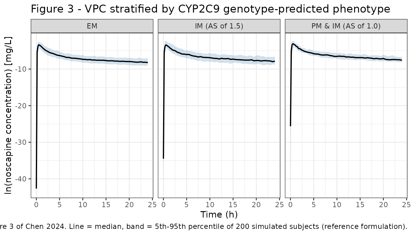
Figure S2 – mean profiles by formulation and phenotype
Figure S2 of the ESM shows the mean concentration-time profiles stratified by formulation and CYP2C9 phenotype. The paper’s summary of it (Sect. 3.2) is that there are “minor differences in Cmax and AUC0-t between the two formulations”, while “subjects with a dysfunctional CYP2C9 allele had a noticeable higher level in both Cmax and AUC0-t” – the formulation effect is small relative to the genotype effect.
sim |>
  group_by(phenotype, formulation, tad) |>
  summarise(mean_dv = mean(dv), .groups = "drop") |>
  ggplot(aes(tad, mean_dv, colour = formulation)) +
  geom_line(linewidth = 0.7) +
  facet_wrap(~phenotype) +
  scale_y_log10() +
  scale_colour_manual(values = c(Reference = "#1b6ca8", Test = "#c1666b")) +
  labs(
    x = "Time (h)", y = "Mean noscapine concentration (ug/L)",
    colour = NULL,
    title = "Figure S2 - mean profiles by formulation and phenotype",
    caption = "Replicates Figure S2 of the Chen 2024 ESM."
  ) +
  theme_bw() +
  theme(legend.position = "bottom")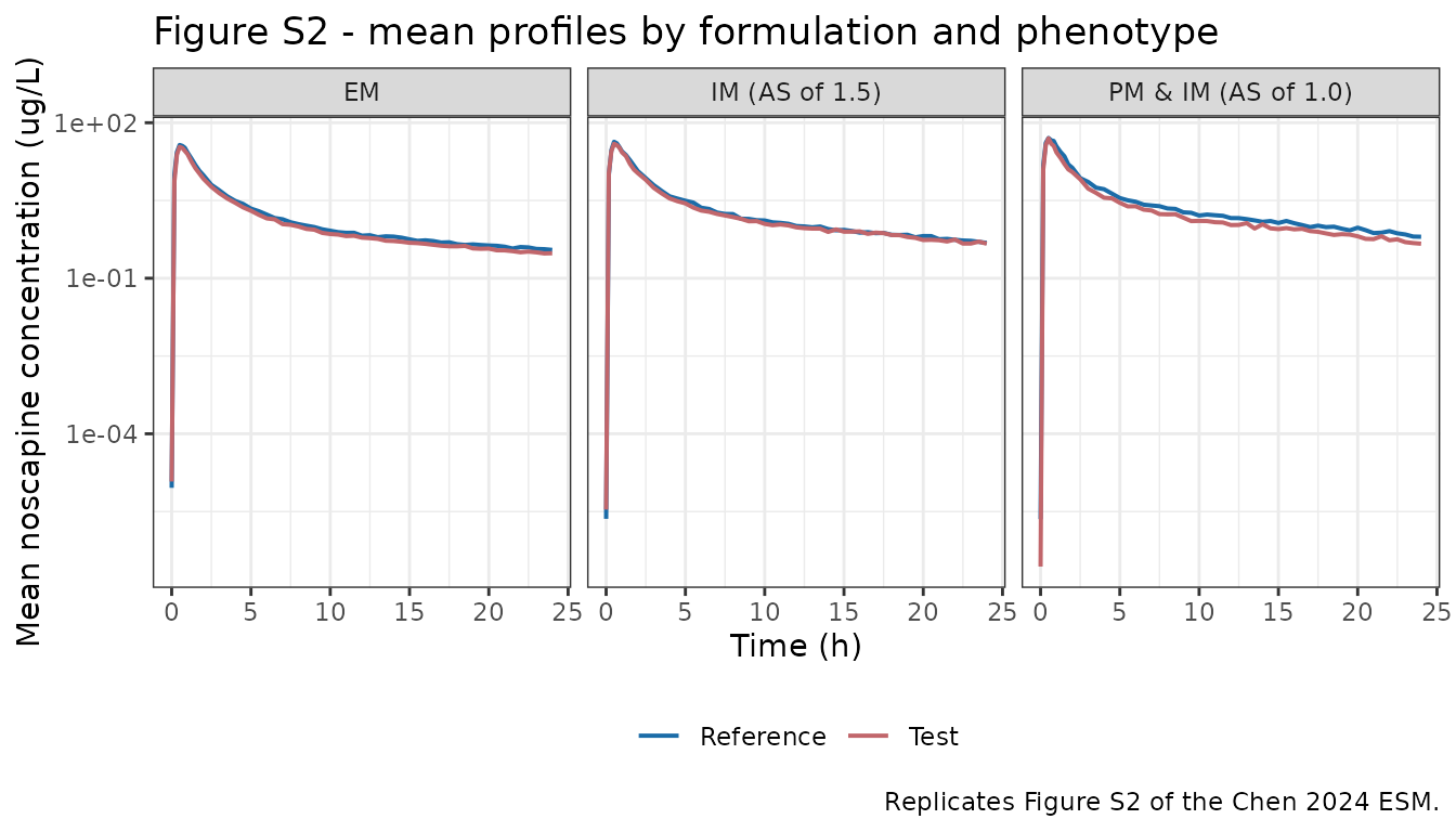
PKNCA validation
The NCA is run on the paper’s own 20-timepoint sampling schedule, per
period, with each period’s time re-based to its own dose so the two
crossover periods present as two profiles per subject. Restricting to
the published schedule matters: lambda_z is estimated from
a window that ends at 24 h, which truncates the model’s true terminal
phase (see the half-life note below).
# Per-period profiles on the paper's schedule, time re-based within period.
nca_conc <- sim |>
  filter(tad %in% obs_pk, !is.na(dv)) |>
  transmute(id, formulation, period, time = tad, Cc = dv)

# Guarantee a time = 0 row per (id, formulation); pre-dose Cc = 0 for an
# extravascular dose. Filtering on `time > 0` or `Cc > 0` here would drop it and
# trigger PKNCA's "AUC range starting before the first measurement" warning.
nca_conc <- bind_rows(
  nca_conc,
  nca_conc |> distinct(id, formulation, period) |> mutate(time = 0, Cc = 0)
) |>
  distinct(id, formulation, time, .keep_all = TRUE) |>
  arrange(id, formulation, time)

nca_dose <- periods |>
  transmute(id, formulation, time = 0, amt = 50)

conc_obj <- PKNCA::PKNCAconc(nca_conc, Cc ~ time | formulation + id)
dose_obj <- PKNCA::PKNCAdose(nca_dose, amt ~ time | formulation + id)

intervals <- data.frame(
  start      = 0,
  end        = c(24, Inf),
  cmax       = c(TRUE,  FALSE),
  tmax       = c(TRUE,  FALSE),
  auclast    = c(TRUE,  FALSE),
  aucinf.obs = c(FALSE, TRUE),
  half.life  = c(FALSE, TRUE)
)

nca_res <- PKNCA::pk.nca(PKNCA::PKNCAdata(conc_obj, dose_obj, intervals = intervals))
Comparison against published NCA
Table 3 of Chen 2024 reports geometric means. For a log-normal
distribution the geometric mean equals the median, which is the
statistic ncaComparisonTable() pools on, so the two are
directly comparable.
published <- tibble::tribble(
  ~formulation, ~cmax, ~tmax, ~auclast, ~aucinf.obs, ~half.life,
  "Test",        36.8,   0.5,     53.1,        57.0,       8.42,
  "Reference",   46.9,   0.5,     64.1,        67.8,       8.29
)

cmp <- nlmixr2lib::ncaComparisonTable(
  simulated = nca_res,
  reference = published,
  by        = "formulation",
  units     = c(cmax = "ug/L", tmax = "h", auclast = "ug*h/L",
                aucinf.obs = "ug*h/L", half.life = "h"),
  tolerance_pct = 20
)

knitr::kable(
  cmp,
  caption = paste("Simulated vs. published NCA (Chen 2024 Table 3).",
                  "* differs from the reference value by more than 20%."),
  digits = 2
)| NCA parameter | formulation | Reference | Simulated | % diff |
|---|---|---|---|---|
| Cmax (ug/L) | Test | 36.8 | 35.4 | -3.7% |
| Cmax (ug/L) | Reference | 46.9 | 44.1 | -6.0% |
| Tmax (h) | Test | 0.5 | 0.67 | +34.0%* |
| Tmax (h) | Reference | 0.5 | 0.67 | +34.0%* |
| AUC0-∞ (obs) (ug*h/L) | Test | 57 | 58.3 | +2.3% |
| AUC0-∞ (obs) (ug*h/L) | Reference | 67.8 | 70.4 | +3.8% |
| AUClast (ug*h/L) | Test | 53.1 | 54.8 | +3.1% |
| AUClast (ug*h/L) | Reference | 64.1 | 64.5 | +0.6% |
| t½ (h) | Test | 8.42 | 8.3 | -1.4% |
| t½ (h) | Reference | 8.29 | 8.18 | -1.3% |
Cmax agrees to within 6%, AUClast and
AUC0-inf to within 4%, and t1/2 to within 1.5%
in both formulations. Note that PKNCA selects each subject’s
lambda_z window automatically and lands on the published
8.3–8.4 h, which independently corroborates the half-life discussion
below.
The starred Tmax row is a sampling-grid
artefact, not a model discrepancy. Tmax is not
interpolated – it can only take a value present in the sampling
schedule, and near the peak that schedule steps in 0.17 h (10 min)
increments: 0.33, 0.5, 0.67, 0.83. The typical-value profile peaks at
0.505 h (Gate 1 above, on a 0.01 h grid), squarely between two adjacent
sampling times, so per-subject Tmax splits between 0.5 and
0.67 h and the median lands on the upper of the two. The absolute
discrepancy is one grid step – 0.17 h – which
ncaComparisonTable()’s percentage measure inflates to 34%
only because the denominator is itself small. The published
Tmax range (0.17–2.0 h, Table 3) brackets the simulated
values throughout. No parameter was adjusted.
Test / reference ratio
The bioequivalence conclusion rests on the T/R ratio, which the model
carries entirely in F1. Because the crossover is simulated
with shared between-subject etas, the ratio can be formed within subject
exactly as the trial analysed it.
tr <- nca_conc |>
  group_by(id, formulation) |>
  summarise(cmax = max(Cc),
            auclast = trapz(time, Cc),
            .groups = "drop") |>
  tidyr::pivot_longer(c(cmax, auclast), names_to = "parameter") |>
  tidyr::pivot_wider(names_from = formulation, values_from = value) |>
  group_by(parameter) |>
  summarise(tr_ratio = exp(mean(log(Test / Reference))), .groups = "drop") |>
  mutate(
    published = c(auclast = 0.827, cmax = 0.784)[parameter],
    published_ci = c(auclast = "0.748-0.915", cmax = "0.662-0.929")[parameter]
  )

tr |>
  rename("Parameter"            = parameter,
         "Simulated T/R"        = tr_ratio,
         "Published T/R"        = published,
         "Published 94.12% CI"  = published_ci) |>
  knitr::kable(digits = 3,
caption = "Within-subject test/reference ratio against Table 3.")| Parameter | Simulated T/R | Published T/R | Published 94.12% CI |
|---|---|---|---|
| auclast | 0.830 | 0.827 | 0.748-0.915 |
| cmax | 0.831 | 0.784 | 0.662-0.929 |
The simulated AUC ratio reproduces
F1 = 0.828 and sits inside the published 94.12% CI for both
parameters. The Cmax ratio is also close to
F1: because the zero-order input duration D1
does not differ by formulation (Sect. 3.3.2 – “only apparent
bioavailability differed between test and reference preparations”), the
model scales the whole profile, so its Cmax ratio is nearer
to F1 than the observed 0.784.
Half-life and the 24-hour sampling window
The model’s true terminal half-life is longer than the published value, and the difference is an estimator artefact rather than a transcription error. Sampling stops at 24 h, so a log-linear regression over the observable window cannot reach the model’s slowest eigenvalue.
typ <- rxode2::rxSolve(mod, typical_events(times = obs_pk),
                       omega = NA, returnType = "data.frame",
                       atol = 1e-10, rtol = 1e-10) |>
  filter(Cc > 0)
long <- rxode2::rxSolve(mod, typical_events(times = seq(24, 400, by = 0.5)),
                        omega = NA, returnType = "data.frame",
                        atol = 1e-10, rtol = 1e-10)
# Keep Cc >= 1e-6 * Cmax (the peak is in `typ`; `long` starts at 24 h): below that the ODE integrator has no relative accuracy left.
long <- filter(long, Cc >= 1e-6 * max(typ$Cc))

fit_thalf <- function(d) {
  log(2) / -stats::coef(stats::lm(log(Cc) ~ time, data = d))[[2]]
}

tibble::tibble(
  window = c("4-24 h", "6-24 h", "9-24 h", "12-24 h", "24-400 h (true terminal)"),
  t_half = c(fit_thalf(filter(typ, time >= 4, time <= 24)),
             fit_thalf(filter(typ, time >= 6, time <= 24)),
             fit_thalf(filter(typ, time >= 9, time <= 24)),
             fit_thalf(filter(typ, time >= 12, time <= 24)),
             fit_thalf(long))
) |>
  rename("Regression window" = window, "t1/2 (h)" = t_half) |>
  knitr::kable(digits = 2,
               caption = paste("Typical-value terminal half-life by regression window.",
"Table 3 reports 8.42 h (test) and 8.29 h (reference)."))| Regression window | t1/2 (h) |
|---|---|
| 4-24 h | 7.11 |
| 6-24 h | 8.85 |
| 9-24 h | 10.89 |
| 12-24 h | 11.89 |
| 24-400 h (true terminal) | 12.47 |
A 6–24 h window gives 8.9 h against the published 8.3–8.4 h, while the model’s true terminal half-life is about 12.5 h. The paper itself notes that its half-life is “approximately twice the previously reported value of 4.5 h” and attributes the difference to a more sensitive assay – the same truncation mechanism, one generation earlier.
Assumptions and deviations
-
Residual-error scale. Table 4 reports “Additive
error 0.0420” in the logarithmic domain without stating whether the
figure is the NONMEM
$SIGMAvariance or a standard deviation. It is read here as a variance, soexpSd = sqrt(0.0420) = 0.2049(a 20.7% residual CV). Maintainer-ratified reading. Supporting evidence: the NONMEM$SIGMAconvention; this being the only variability row left in raw NONMEM units while every other was converted to CV%; the reported 2.4% RSE matching thesqrt(2/1920) = 3.2%expected of a variance estimated from 1920 observations rather than the ~1.6% an SD would give; and a 4.2% residual CV being implausibly tight for LC-MS/MS plasma data. -
IIV CV% convention. Table 4’s CV% values are
back-transformed as
omega^2 = log(1 + CV^2), the correct conversion for the exponential IIV model of Sect. 2.4.1. Gate 3 above confirms this against the paper’s own observed AUC CV; the alternativeomega = CVreading overshoots it. The IOV values, reported under a header that gives only “(%)”, are converted the same way for consistency with the IIV rows. -
Unreported IIV covariances are zero. Table 4
reports three covariances (
D1–CL/F,D1–V/F,D1–F1). The remaining three off-diagonals of the four-eta block were not in the NONMEM$OMEGA BLOCKand are encodedfixed(0). The resulting matrix is positive definite (implied correlations 0.15, -0.47, 0.36). -
Inter-occasion variability across two occasions.
nlmixr2 has no equivalent of NONMEM’s
$OMEGA BLOCK(1) SAME, so occasion 2 receives its own eta with the variance fixed equal to the occasion-1 estimate, following theChen_2023_nemonoxacin.RandJonsson_2011_ethambutol.Rprecedent. PassingOCC = 1gives a single-occasion simulation. -
Mixed apparent and physiologic scales in the liver
arm.
Qh(55 L/h) andVh(1.5 L) are true physiologic constants while every plasma-side volume and clearance is apparent (/F). The liver state therefore holds an apparent amount. This is the paper’s own construction, not a transcription choice, and it is benign for prediction: Gate 1 shows total exposure isDose * F / (CL/F)regardless, so the liver arm sets only the shape of the absorption phase. The paper’s Table S2 sensitivity analysis reached the same conclusion empirically. -
Covariate centring values.
CL/Fis normalised to 77.3 kg, the cohort mean weight, andQp1/Fto 29.0 years, the cohort median age – both taken verbatim from the Sect. 3.3.2 equations rather than assumed. Note the paper mixes a mean and a median across the two equations, and that the weight exponent 1.34 was estimated, not fixed at an allometric 0.75. -
CL/Fstrata are discrete, not activity-score-proportional. The three publishedCL/Fvalues are not proportional to the CPIC activity score (531/958 = 0.554 and 343/958 = 0.358 against activity-score ratios of 0.75 and 0.50), so the phenotype is encoded as two mutually exclusive binary indicators. A continuous activity-score covariate cannot reproduce the published typical values. -
Virtual-cohort covariate distributions. Weight is
assigned from deterministic normal quantiles (mean 77.3 kg, SD 12.7,
truncated to 54.3–107 kg per Table 1). Age is right-skewed in the source
(mean 33, median 29, range 19–65), which Table 1 gives only as summary
statistics; a log-normal matching both the reported median and mean is
used, truncated to the reported range. Genotype strata follow the Table
2 proportions exactly. Sex, height, BMI, liver-function and
renal-function markers are not model covariates (they were screened and
not retained) and are omitted from the cohort; they are documented in
the model file’s
covariatesDataExcluded. - Washout length. The trial used 6–14 days; 240 h (10 days, about 19 model half-lives) is used so period-2 profiles start from negligible carryover.
-
Tmaxcomparison is grid-limited. The published and simulatedTmaxdiffer by exactly one sampling interval (0.17 h), which registers as a >20% flag in the NCA comparison table purely becauseTmaxis small. The typical-value peak is at 0.505 h against a published median of 0.5 h. See the note under the comparison table. -
CmaxT/R ratio. The model predicts aCmaxT/R ratio nearF1 = 0.828whereas the observed ratio was 0.784, because no absorption-rate parameter differs by formulation in the published model. This is a property of the published structure, not a deviation introduced here; no parameter was tuned. -
Half-life comparison window. The published 8.3–8.4
h half-life is reproduced only when
lambda_zis regressed over the paper’s own truncated sampling window; the model’s true terminal half-life is about 12.5 h. See the half-life section above. - No erratum. A search of the journal landing page and PubMed found no erratum, corrigendum or author correction for this article.
- Supplement. The ESM was not required for extraction: every final parameter value is in main-text Table 4, and both covariate equations are in Sect. 3.3.2. The ESM holds model-development attempts (Table S1), the liver-compartment sensitivity analysis (Table S2) and diagnostic plots (Figs. S1–S7), which are referenced above but supply no extracted value.