Vigabatrin (Nielsen 2015)
Source:vignettes/articles/Nielsen_2015_vigabatrin.Rmd
Nielsen_2015_vigabatrin.RmdModel and source
- Citation: Nielsen JC, Hutmacher MM, Wesche DL, Tolbert D, Patel M, Kowalski KG. Population dose-response analysis of daily seizure count following vigabatrin therapy in adult and pediatric patients with refractory complex partial seizures. J Clin Pharmacol. 2015;55(1):81-92.
- Article: https://doi.org/10.1002/jcph.378
This is a population dose-response (PD) count model,
not a popPK model. Daily seizure counts from five randomized controlled
trials (two adult, three pediatric) are described by a negative-binomial
distribution whose mean rate lambda is the product of three
terms: a baseline rate that rises with decreasing age, a non-drug time
(“placebo”) effect that approaches an asymptote after the first
randomized dose, and a quadratic drug effect.
There is no PK model and no ODE state at all.
Pediatric PK data were unavailable when the analysis was done, so the
authors estimated an exposure surrogate in-model – normalized
dosage, the actual total daily dosage rescaled to a
60-kg-equivalent via (WT/60)^-0.608. Drug exposure
therefore enters through the covariate DOSE_VGB_MGD rather
than through a concentration.
ui <- rxode2::rxode(readModelDb("Nielsen_2015_vigabatrin"))
mod_typical <- rxode2::zeroRe(ui)
#> Warning: No sigma parameters in the model
Population
pop <- ui$population
knitr::kable(
  data.frame(field = names(pop),
             value = vapply(pop, function(x) paste(
               if (is.null(names(x))) x else paste0(names(x), "=", x),
               collapse = "; "), character(1))),
  row.names = FALSE,
  caption = "population metadata (Nielsen 2015 Tables 1 and 2)."
)| field | value |
|---|---|
| species | human |
| n_subjects | 621 |
| n_studies | 5 |
| age_range | 3-63 years (median 24; pediatric median 11, adult median 33) |
| weight_range | 12-136 kg (median 62; pediatric median 44, adult median 70) |
| sex_female_pct | 53.6 |
| race_ethnicity | White=91.5; Black=5.5; Asian=0.6; Other=2.4 |
| disease_state | Refractory complex partial seizures (rCPS), with or without secondary generalization, on a stable regimen of one or two background antiepileptic drugs. Patients with generalized epilepsy, progressive neurological disorders, treatable causes of seizures or non-epileptic seizures were excluded (Nielsen 2015 Table 1). |
| dose_range | Adults (studies 24, 25): placebo or vigabatrin 1, 3 or 6 g/day. Pediatrics (study 118): placebo or 20, 60 or 100 mg/kg/day, with the dosing weight capped at 60 kg. Pediatrics (studies 192, 221): placebo or weight-banded 0.5-1.5 g/day (10-15 kg), 0.5-2.0 g/day (16-30 kg), 1.0-3.0 g/day (31-50 kg), 1.0-4.0 g/day (over 50 kg). Twice-daily and titrated in all five studies. |
| regions | not reported |
| biomarkers | Daily seizure count from patient diaries. 41,282 daily records from 356 adults and 70,886 daily records from 265 pediatric patients (112,168 records total). Study phases: baseline run-in 6-10 weeks (pediatric) or 10 weeks (adult); dosage titration 6-10 weeks (pediatric) or 4-6 weeks (adult); maintenance 7-8 weeks (pediatric) or 12 weeks (adult). |
| notes | Demographics from Nielsen 2015 Table 2 (pooled column); study designs and enrolment from Table 1. The three pediatric studies were suspended before completing planned enrolment for administrative reasons and were individually underpowered for dose response, which is the stated motivation for the pooled analysis. Model fitted in NONMEM 7.2 with the Laplace method; final objective function 195069.298, condition number 149 (Table 3). |
Source trace
Per-parameter origins are recorded as in-file comments beside each
ini() entry in
inst/modeldb/specificDrugs/Nielsen_2015_vigabatrin.R.
Collected here:
| nlmixr2 parameter | Value | Nielsen 2015 source |
|---|---|---|
lrbase |
-1.070 | Table 3 “LN lambda - Adults” (SE 0.0394); Eq. 10b |
e_age_rbase |
-0.4180 | Table 3 “Age on LN lambda” (SE 0.0592); Eq. 10b |
lovdp |
0.0924 | Table 3 “LN OVDP - Adults” (SE 0.0195); Eq. 1 |
e_study_118_ovdp |
-0.6710 | Table 3 “D LN OVDP - Study 118” (SE 0.0412) |
e_study_192_ovdp |
-0.9400 | Table 3 “D LN OVDP - Study 192” (SE 0.0743) |
e_study_221_ovdp |
-1.4200 | Table 3 “D LN OVDP - Study 221” (SE 0.0730) |
astime |
-0.1560 | Table 3 “AS - Adults” (SE 0.2430); Eq. 10c |
e_study_118_astime |
0.1200 | Table 3 “D AS - Study 118” (SE 0.4060) |
e_study_192_astime |
-0.5840 | Table 3 “D AS - Study 192” (SE 0.3780) |
e_study_221_astime |
-0.3740 | Table 3 “D AS - Study 221” (SE 0.3640) |
lktime |
-5.000 | Table 3 “LN k” (SE 0.2780); Eq. 10d |
laquad |
-1.2900 | Table 3 “LN a” (SE 0.2280); Eq. 10f |
lblin |
-0.1220 | Table 3 “LN b” (SE 0.1180); Eq. 10f |
e_wt_dosenorm |
-0.6080 | Table 3 “WT on DNORM” (SE 0.1740); Eq. 10e |
bc_shape |
0.7450 | Table 3 “SHAPE - Adults” (SE 0.1040); Eq. 9 |
lsd_rbase |
-0.3190 | Table 3 “LN v - lambda - Adults” (SE 0.0552) |
e_study_118_sd_rbase |
0.5860 | Table 3 “D LN v - lambda - Study 118” (SE 0.0867) |
e_study_192_sd_rbase |
0.8860 | Table 3 “D LN v - lambda - Study 192” (SE 0.1220) |
e_study_221_sd_rbase |
0.3580 | Table 3 “D LN v - lambda - Study 221” (SE 0.0989) |
etaastime |
var 4.0068 | Table 3 “LN v - AS” = 0.6940 (SE 0.2130); var = exp(2 x 0.694) |
etalblin |
var 0.7603 | Table 3 “LN v - b” = -0.1370 (SE 0.0699); var = exp(2 x -0.137) |
etalrbase |
fixed 1 | standard normal; rescaled in model() by the
study-dependent SD |
| negative-binomial likelihood | – | Eq. 1 |
| multiplicative rate structure | – | Eq. 2, Eq. 10a |
A transcription hazard worth recording. The
publisher’s PDF drops the minus sign in front of several printed
quantities, and every equation in this paper is lost by
plain-text extraction of the PDF. Two signs matter and were both
recovered from Table 3 and then confirmed against the paper’s own
arithmetic (see the checks below): the exponent in Eq. 10e is
negative (-0.608), and the drug-effect polynomial is
+a x^2 - b x. The indicator in Eq. 10d is
I(DAY >= 1), not “day 1 only”; the subscript
>= is dropped by every text extractor and was confirmed
by rendering the page as an image.
Mechanistic structure
At the typical value the mean daily seizure rate for patient on day is
with
and the observation is negative-binomial with mean and overdispersion , so that .
Closed-form cross-check of the typical values
An independent reimplementation of Eq. 10a-10f in plain R, compared
against rxSolve on the packaged model. Both sides use the
same published constants but share no code, so this checks that the
model file evaluates the source equations.
TH <- list(lrbase = -1.07, e_age = -0.418, astime = -0.156,
           d118 = 0.12, d192 = -0.584, d221 = -0.374,
           lktime = -5, laquad = -1.29, lblin = -0.122, e_wt = -0.608)

closed_lambda <- function(AGE, WT, DOSE, tday, s118 = 0, s192 = 0, s221 = 0) {
  rbase <- exp(TH$lrbase + TH$e_age * (log(AGE) - log(24)))
  AS <- TH$astime + TH$d118 * s118 + TH$d192 * s192 + TH$d221 * s221
  ftime <- exp(AS * (1 - exp(-exp(TH$lktime) * tday)) * (tday >= 1))
  x <- DOSE * (WT / 60)^TH$e_wt / 3000
  fdrug <- exp(exp(TH$laquad) * x^2 - exp(TH$lblin) * x)
  rbase * ftime * fdrug
}

grid <- tibble::tibble(
  label = c("adult baseline", "adult placebo d119", "adult 3 g/d d119",
            "adult 6 g/d d119", "child 118 baseline", "child 118 100 mg/kg d112",
            "child 192 placebo d112", "child 221 placebo d112"),
  AGE   = c(24, 33, 33, 33, 11, 11, 11, 11),
  WT    = c(70, 70, 70, 70, 44, 44, 44, 44),
  DOSE  = c(0, 0, 3000, 6000, 0, 4400, 0, 0),
  tday  = c(0, 119, 119, 119, 0, 112, 112, 112),
  s118  = c(0, 0, 0, 0, 1, 1, 0, 0),
  s192  = c(0, 0, 0, 0, 0, 0, 1, 0),
  s221  = c(0, 0, 0, 0, 0, 0, 0, 1)
)

ev <- grid |>
  dplyr::mutate(id = dplyr::row_number(), time = tday, evid = 0L, amt = 0) |>
  dplyr::transmute(id, time, evid, amt, AGE, WT, DOSE_VGB_MGD = DOSE,
                   STUDY_118 = s118, STUDY_192 = s192, STUDY_221 = s221)

sim <- rxode2::rxSolve(mod_typical, ev, returnType = "data.frame")
#> ℹ omega/sigma items treated as zero: 'etalrbase', 'etaastime', 'etalblin'

cmp <- grid |>
  dplyr::mutate(
    id = dplyr::row_number(),
    lambda_closed = closed_lambda(AGE, WT, DOSE, tday, s118, s192, s221)
  ) |>
  dplyr::left_join(dplyr::select(sim, id, lambda_rxode = lambda), by = "id") |>
  dplyr::mutate(rel_err = abs(lambda_rxode - lambda_closed) / lambda_closed)

knitr::kable(dplyr::select(cmp, label, lambda_closed, lambda_rxode, rel_err),
             digits = c(0, 6, 6, 12),
caption = "Independent closed form vs rxSolve. Both sides evaluate Eq. 10a-10f.")| label | lambda_closed | lambda_rxode | rel_err |
|---|---|---|---|
| adult baseline | 0.343009 | 0.343009 | 0 |
| adult placebo d119 | 0.275506 | 0.275506 | 0 |
| adult 3 g/d d119 | 0.154605 | 0.154605 | 0 |
| adult 6 g/d d119 | 0.136944 | 0.136944 | 0 |
| child 118 baseline | 0.475260 | 0.475260 | 0 |
| child 118 100 mg/kg d112 | 0.230572 | 0.230572 | 0 |
| child 192 placebo d112 | 0.321112 | 0.321112 | 0 |
| child 221 placebo d112 | 0.358904 | 0.358904 | 0 |
Published anchor 1: baseline rate and time-effect half-life
lambda_24 <- closed_lambda(AGE = 24, WT = 70, DOSE = 0, tday = 0)
thalf_time <- log(2) / exp(TH$lktime)

knitr::kable(
  data.frame(
    quantity = c("Typical baseline rate, 24-year-old (seizures/day)",
                 "Time-effect half-life (days)"),
    model    = c(round(lambda_24, 4), round(thalf_time, 1)),
    published = c("0.343", "approximately 100")
  ),
  caption = "Nielsen 2015 Results, Covariate Model."
)| quantity | model | published |
|---|---|---|
| Typical baseline rate, 24-year-old (seizures/day) | 0.343 | 0.343 |
| Time-effect half-life (days) | 102.900 | approximately 100 |
Published anchor 2: the normalized-dosage equivalence
The paper states that “a 20-kg patient receiving a total daily dosage of 1.54 g, a 60-kg patient receiving a total daily dosage of 3 g, and a 100-kg patient receiving a total daily dosage of 4.09 g would have the same normalized total daily dosage”. This is the check that pins the sign of the Eq. 10e exponent.
eq_ev <- data.frame(
  id = 1:3, time = 0, evid = 0L, amt = 0,
  AGE = 33, WT = c(20, 60, 100), DOSE_VGB_MGD = c(1540, 3000, 4090),
  STUDY_118 = 0, STUDY_192 = 0, STUDY_221 = 0
)
eq_sim <- rxode2::rxSolve(mod_typical, eq_ev, returnType = "data.frame")
#> ℹ omega/sigma items treated as zero: 'etalrbase', 'etaastime', 'etalblin'

knitr::kable(
  data.frame(WT_kg = c(20, 60, 100), dose_mg_per_day = c(1540, 3000, 4090),
             dosenorm_mg = round(eq_sim$dosenorm, 1)),
  caption = "Normalized dosage is equal across the paper's three worked patients."
)| WT_kg | dose_mg_per_day | dosenorm_mg |
|---|---|---|
| 20 | 1540 | 3003.4 |
| 60 | 3000 | 3000.0 |
| 100 | 4090 | 2998.1 |
# The paper's doses are printed to 3 significant figures, so the three
# normalized dosages agree to within that rounding, not exactly.
stopifnot(nrow(eq_sim) == 3L,
          max(abs(eq_sim$dosenorm - 3000)) < 5)
If the exponent were taken as +0.608 (the sign as
printed in Eq. 10e, whose minus the PDF drops), the same three patients
would give normalized dosages of 790, 3000 and 5580 mg – not equal, and
so falsified by the paper’s own sentence.
Published anchor 3: the dose-response curve (Figure 1)
dr_ev <- data.frame(
  id = seq_len(121), time = 0, evid = 0L, amt = 0,
  AGE = 24, WT = 60,
  DOSE_VGB_MGD = seq(0, 6000, length.out = 121),
  STUDY_118 = 0, STUDY_192 = 0, STUDY_221 = 0
)
dr <- rxode2::rxSolve(mod_typical, dr_ev, returnType = "data.frame") |>
  dplyr::mutate(pct_reduction = 100 * (1 - fdrug))
#> ℹ omega/sigma items treated as zero: 'etalrbase', 'etaastime', 'etalblin'

ggplot(dr, aes(dosenorm / 1000, pct_reduction)) +
  geom_line(colour = "steelblue", linewidth = 1) +
  geom_point(data = data.frame(d = c(1, 3, 6), p = c(23.2, 45.6, 48.5)),
             aes(d, p), colour = "firebrick", size = 2.5, inherit.aes = FALSE) +
  labs(x = "Normalized total daily dosage (g/day)",
       y = "Reduction in mean seizure rate (%)",
       title = "Vigabatrin normalized dose-response (typical value)",
       subtitle = "Red points are the reductions quoted in the paper at 1, 3 and 6 g/day.")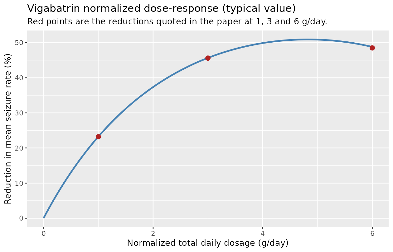
Replicates Figure 1 of Nielsen 2015: typical-value normalized dose-response.
At a 60-kg reference weight normalized dosage equals actual dosage, so these are directly the paper’s quoted numbers:
red <- function(g) 100 * (1 - closed_lambda(24, 60, g * 1000, 0) /
                            closed_lambda(24, 60, 0, 0))

# Dose giving half the response seen at 6 g/day (paper: 1.065 g/day).
half6 <- uniroot(function(d) red(d / 1000) - red(6) / 2, c(1, 6000))$root

anchors <- data.frame(
  quantity  = c("Reduction at 1 g/day (%)", "Reduction at 3 g/day (%)",
                "Reduction at 6 g/day (%)", "Dose at half the 6 g/day response (g/day)"),
  model     = round(c(red(1), red(3), red(6), half6 / 1000), 4),
  published = c(23.2, 45.6, 48.5, 1.065)
)
knitr::kable(anchors, caption = "Nielsen 2015 Abstract and Discussion.")| quantity | model | published |
|---|---|---|
| Reduction at 1 g/day (%) | 23.2383 | 23.200 |
| Reduction at 3 g/day (%) | 45.6583 | 45.600 |
| Reduction at 6 g/day (%) | 48.7889 | 48.500 |
| Dose at half the 6 g/day response (g/day) | 1.0655 | 1.065 |
stopifnot(
  abs(red(1) - 23.2) < 0.1,
  abs(red(3) - 45.6) < 0.1,
  # The paper's own 'half the 6 g/day response at 1.065 g/day' statement is the
  # tighter constraint and it is met to 4 significant figures.
  abs(half6 / 1000 - 1.065) < 0.002
)
The 6 g/day row is the one published number this model does not reproduce: the equation gives 48.79% where the abstract says 48.5%. See “Assumptions and deviations” – the paper’s own half-response statement agrees with the equation, not with 48.5%.
Published anchor 4: reproducing Table 4 (posterior predictive check)
Table 4 of the paper reports, for each study / dose / treatment-period cell, the observed median of the mean monthly (28-day) seizure frequency together with the 90% prediction interval generated by the authors’ own final model. A correct transcription of the model must place its typical-value prediction inside those published intervals.
Covariates are the paper’s own medians (Table 2: adults age 33 / 70 kg, pediatrics age 11 / 44 kg) and the durations come from the Table 1 study designs.
# Treatment duration at "end of study" = titration + maintenance (Table 1).
# Adults (studies 24, 25): titration 4-6 weeks, maintenance 12 weeks.
# Pediatrics (118, 192, 221): titration 6-10 weeks, maintenance 7-8 weeks.
T_EOS_ADULT <- (5 + 12) * 7      # 119 days, titration midpoint
T_EOS_PEDS  <- (8 + 7.5) * 7     # 108.5 days, both midpoints

tab4 <- tibble::tribble(
  ~study, ~arm,            ~period,  ~dose_mg, ~obs,  ~lo,   ~hi,   ~gated,
  24,  "Placebo",           "Baseline",     0, 8.11,  7.12, 10.1,  TRUE,
  24,  "Placebo",           "End of study", 0, 7.37,  6.47, 12.5,  TRUE,
  24,  "Vigabatrin 3 g/day","Baseline",  3000, 8.84,  7.37, 10.3,  TRUE,
  24,  "Vigabatrin 3 g/day","End of study",3000, 4.79, 2.95,  5.89, TRUE,
  25,  "Placebo",           "Baseline",     0, 9.33,  6.88, 10.8,  TRUE,
  25,  "Placebo",           "End of study", 0, 8.65,  5.89, 13.3,  TRUE,
  25,  "Vigabatrin 1 g/day","Baseline",  1000, 9.82,  6.88, 10.8,  TRUE,
  25,  "Vigabatrin 1 g/day","End of study",1000, 7.54, 3.96,  9.66, TRUE,
  25,  "Vigabatrin 3 g/day","Baseline",  3000, 7.86,  6.88, 11.3,  TRUE,
  25,  "Vigabatrin 3 g/day","End of study",3000, 3.50, 2.50,  6.94, TRUE,
  25,  "Vigabatrin 6 g/day","Baseline",  6000, 8.84,  6.88, 11.3,  TRUE,
  25,  "Vigabatrin 6 g/day","End of study",6000, 4.42, 1.96,  7.00, TRUE,
  118, "Placebo",           "Baseline",     0, 19.2,  9.00, 24.6,  TRUE,
  118, "Placebo",           "End of study", 0, 14.9,  8.29, 27.6,  TRUE,
  118, "Vigabatrin 20 mg/kg/day", "Baseline",   44*20,  16.2, 8.35, 23.6, TRUE,
  118, "Vigabatrin 20 mg/kg/day", "End of study",44*20, 10.2, 5.11, 17.4, TRUE,
  118, "Vigabatrin 60 mg/kg/day", "Baseline",   44*60,   8.35, 8.11, 21.3, TRUE,
  118, "Vigabatrin 60 mg/kg/day", "End of study",44*60,  7.50, 2.58, 10.5, TRUE,
  118, "Vigabatrin 100 mg/kg/day","Baseline",   44*100, 13.4, 9.12, 24.4, TRUE,
  118, "Vigabatrin 100 mg/kg/day","End of study",44*100, 2.75, 2.63, 11.8, TRUE,
  192, "Placebo",           "Baseline",     0, 7.16,  6.37, 26.7,  TRUE,
  192, "Placebo",           "End of study", 0, 4.00,  4.00, 21.9,  TRUE,
  192, "Vigabatrin 0.5-4 g/day","Baseline",  0, 13.3,  6.84, 26.5,  TRUE,
  192, "Vigabatrin 0.5-4 g/day","End of study", NA, 3.31, 1.99, 12.1, FALSE,
  221, "Placebo",           "Baseline",     0, 16.2, 10.6,  21.6,  TRUE,
  221, "Placebo",           "End of study", 0, 14.7,  7.91, 20.7,  TRUE,
  221, "Vigabatrin 0.5-4 g/day","Baseline",  0,  8.00, 9.33, 20.0,  TRUE,
  221, "Vigabatrin 0.5-4 g/day","End of study", NA, 7.33, 2.33,  8.39, FALSE
)
Two cells are not gated: studies 192 and 221 dosed by weight band, so the “0.5-4 g/day” active arm has no single end-of-study dose. Their baseline rows are gated, because at baseline the dose is zero for every arm and the drug term is exactly 1. For the two ungated cells a predicted band across the 1.0-3.0 g/day band applicable to a 44-kg child is reported instead.
tab4 <- tab4 |>
  dplyr::mutate(
    peds  = study %in% c(118, 192, 221),
    AGE   = ifelse(peds, 11, 33),
    WT    = ifelse(peds, 44, 70),
    tday  = ifelse(period == "Baseline", 0,
                   ifelse(peds, T_EOS_PEDS, T_EOS_ADULT)),
    dose_eff = ifelse(period == "Baseline", 0, dose_mg),
    s118 = as.integer(study == 118),
    s192 = as.integer(study == 192),
    s221 = as.integer(study == 221),
    pred = 28 * closed_lambda(AGE, WT, dose_eff, tday, s118, s192, s221),
    in_pi = !is.na(pred) & pred >= lo & pred <= hi
  )

knitr::kable(
  tab4 |>
    dplyr::filter(gated) |>
    dplyr::transmute(Study = study, Arm = arm, Period = period,
                     `Model (per 28 d)` = round(pred, 2),
                     `Observed median` = obs,
                     `90% PI` = paste0(lo, ", ", hi),
                     `Inside PI` = ifelse(in_pi, "yes", "NO")),
  caption = "Reproduction of Nielsen 2015 Table 4 (gated cells)."
)| Study | Arm | Period | Model (per 28 d) | Observed median | 90% PI | Inside PI |
|---|---|---|---|---|---|---|
| 24 | Placebo | Baseline | 8.41 | 8.11 | 7.12, 10.1 | yes |
| 24 | Placebo | End of study | 7.71 | 7.37 | 6.47, 12.5 | yes |
| 24 | Vigabatrin 3 g/day | Baseline | 8.41 | 8.84 | 7.37, 10.3 | yes |
| 24 | Vigabatrin 3 g/day | End of study | 4.33 | 4.79 | 2.95, 5.89 | yes |
| 25 | Placebo | Baseline | 8.41 | 9.33 | 6.88, 10.8 | yes |
| 25 | Placebo | End of study | 7.71 | 8.65 | 5.89, 13.3 | yes |
| 25 | Vigabatrin 1 g/day | Baseline | 8.41 | 9.82 | 6.88, 10.8 | yes |
| 25 | Vigabatrin 1 g/day | End of study | 6.05 | 7.54 | 3.96, 9.66 | yes |
| 25 | Vigabatrin 3 g/day | Baseline | 8.41 | 7.86 | 6.88, 11.3 | yes |
| 25 | Vigabatrin 3 g/day | End of study | 4.33 | 3.50 | 2.5, 6.94 | yes |
| 25 | Vigabatrin 6 g/day | Baseline | 8.41 | 8.84 | 6.88, 11.3 | yes |
| 25 | Vigabatrin 6 g/day | End of study | 3.83 | 4.42 | 1.96, 7 | yes |
| 118 | Placebo | Baseline | 13.31 | 19.20 | 9, 24.6 | yes |
| 118 | Placebo | End of study | 13.06 | 14.90 | 8.29, 27.6 | yes |
| 118 | Vigabatrin 20 mg/kg/day | Baseline | 13.31 | 16.20 | 8.35, 23.6 | yes |
| 118 | Vigabatrin 20 mg/kg/day | End of study | 9.88 | 10.20 | 5.11, 17.4 | yes |
| 118 | Vigabatrin 60 mg/kg/day | Baseline | 13.31 | 8.35 | 8.11, 21.3 | yes |
| 118 | Vigabatrin 60 mg/kg/day | End of study | 6.96 | 7.50 | 2.58, 10.5 | yes |
| 118 | Vigabatrin 100 mg/kg/day | Baseline | 13.31 | 13.40 | 9.12, 24.4 | yes |
| 118 | Vigabatrin 100 mg/kg/day | End of study | 6.46 | 2.75 | 2.63, 11.8 | yes |
| 192 | Placebo | Baseline | 13.31 | 7.16 | 6.37, 26.7 | yes |
| 192 | Placebo | End of study | 9.07 | 4.00 | 4, 21.9 | yes |
| 192 | Vigabatrin 0.5-4 g/day | Baseline | 13.31 | 13.30 | 6.84, 26.5 | yes |
| 221 | Placebo | Baseline | 13.31 | 16.20 | 10.6, 21.6 | yes |
| 221 | Placebo | End of study | 10.11 | 14.70 | 7.91, 20.7 | yes |
| 221 | Vigabatrin 0.5-4 g/day | Baseline | 13.31 | 8.00 | 9.33, 20 | yes |
gated <- dplyr::filter(tab4, gated)
# Guard that the gate has rows to test (a zero-row all() is vacuously TRUE).
stopifnot(nrow(gated) == 26L, !anyNA(gated$pred), all(gated$in_pi))
cat(sprintf("%d of %d gated Table 4 cells inside the published 90%% PI\n",
            sum(gated$in_pi), nrow(gated)))
#> 26 of 26 gated Table 4 cells inside the published 90% PI
band <- tab4 |>
  dplyr::filter(!gated) |>
  dplyr::rowwise() |>
  dplyr::mutate(
    pred_lo = 28 * closed_lambda(AGE, WT, 3000, tday, s118, s192, s221),
    pred_hi = 28 * closed_lambda(AGE, WT, 1000, tday, s118, s192, s221)
  ) |>
  dplyr::ungroup()

knitr::kable(
  band |>
    dplyr::transmute(Study = study, Period = period,
                     `Model band, 1-3 g/day` =
                       paste0(round(pred_lo, 2), " to ", round(pred_hi, 2)),
                     `Observed median` = obs,
                     `90% PI` = paste0(lo, ", ", hi)),
  caption = "Ungated cells: weight-banded dosing, shown as a predicted band."
)| Study | Period | Model band, 1-3 g/day | Observed median | 90% PI |
|---|---|---|---|---|
| 192 | End of study | 4.65 to 6.64 | 3.31 | 1.99, 12.1 |
| 221 | End of study | 5.19 to 7.4 | 7.33 | 2.33, 8.39 |
# The whole band lies inside the published PI in both cells, so the ungated
# rows corroborate rather than merely abstain.
stopifnot(nrow(band) == 2L,
          all(band$pred_lo >= band$lo), all(band$pred_hi <= band$hi))
Sensitivity to the assumed treatment duration
Table 1 gives titration and maintenance as ranges, so “end of study” is an interval, not a point. Because the time effect has a half-life near 103 days the prediction moves very little across that interval – and the gate holds throughout it.
dur_grid <- expand.grid(
  adult = c((4 + 12) * 7, (6 + 12) * 7),
  peds  = c((6 + 7) * 7,  (10 + 8) * 7)
)

worst <- vapply(seq_len(nrow(dur_grid)), function(k) {
  g <- gated |>
    dplyr::mutate(
      tday2 = ifelse(period == "Baseline", 0,
                     ifelse(peds, dur_grid$peds[k], dur_grid$adult[k])),
      pred2 = 28 * closed_lambda(AGE, WT, dose_eff, tday2, s118, s192, s221)
    )
  sum(g$pred2 >= g$lo & g$pred2 <= g$hi)
}, numeric(1))

knitr::kable(
  cbind(dur_grid, cells_inside_PI = worst, of = nrow(gated)),
  caption = "Gated cells inside the 90% PI across the full plausible duration range."
)| adult | peds | cells_inside_PI | of |
|---|---|---|---|
| 112 | 91 | 26 | 26 |
| 126 | 91 | 26 | 26 |
| 112 | 126 | 26 | 26 |
| 126 | 126 | 26 | 26 |
Time course of the non-drug (placebo) effect
tc <- expand.grid(tday = seq(0, 180, by = 2),
                  study = c("Adults (24, 25)", "Study 118", "Study 192", "Study 221"),
                  stringsAsFactors = FALSE) |>
  dplyr::mutate(
    AS = TH$astime + TH$d118 * (study == "Study 118") +
      TH$d192 * (study == "Study 192") + TH$d221 * (study == "Study 221"),
    ftime = exp(AS * (1 - exp(-exp(TH$lktime) * tday)) * (tday >= 1))
  )

ggplot(tc, aes(tday, 100 * (1 - ftime), colour = study)) +
  geom_line(linewidth = 0.9) +
  labs(x = "Days after the first randomized dose",
       y = "Reduction in seizure rate from time effects (%)",
       colour = NULL,
       title = "Asymptotic non-drug time effect",
       subtitle = "Half-life log(2)/exp(-5) = 103 days, so no arm reaches its asymptote in-trial.")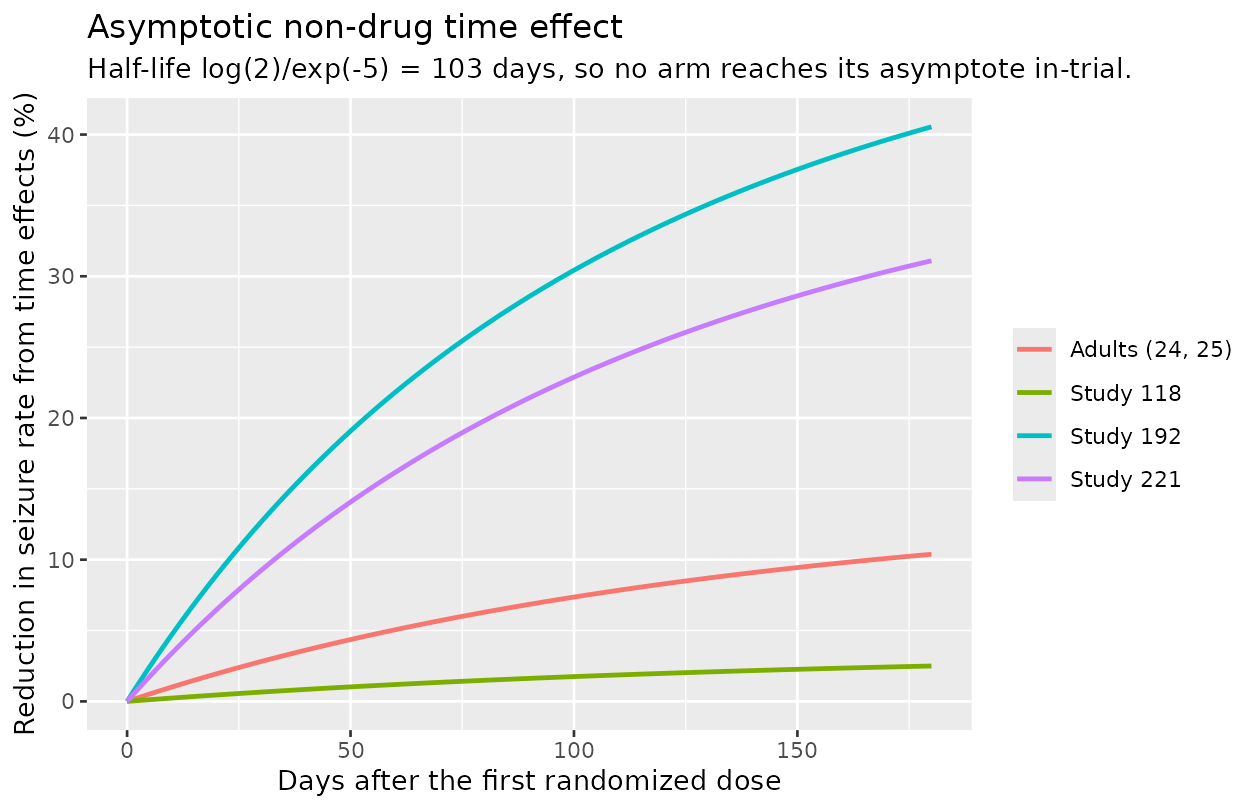
Non-drug time effect by study; the adult curve is the reference.
This reproduces two statements in the paper: the maximum time effect is greater in studies 192 and 221 than in adults, and smaller in study 118; and “most patients would not reach the maximum decline in seizure rate over the duration of the study”.
Negative-binomial sampling and overdispersion
The packaged model declares a Poisson observation likelihood because
rxode2 exposes no negative-binomial endpoint (see “Assumptions and
deviations”). The source overdispersion is exposed as the model variable
ovdp, from which true negative-binomial counts follow with
size = 1/ovdp. This section demonstrates that, and checks
the resulting variance against Eq. 1.
arms <- tibble::tibble(
  arm = c("Adult placebo", "Adult 3 g/day", "Study 118 placebo",
          "Study 118 100 mg/kg/day"),
  AGE = c(33, 33, 11, 11), WT = c(70, 70, 44, 44),
  DOSE = c(0, 3000, 0, 44 * 100),
  s118 = c(0, 0, 1, 1)
)

typ_ev <- arms |>
  dplyr::mutate(id = dplyr::row_number()) |>
  dplyr::transmute(id, time = T_EOS_ADULT, evid = 0L, amt = 0,
                   AGE, WT, DOSE_VGB_MGD = DOSE,
                   STUDY_118 = s118, STUDY_192 = 0, STUDY_221 = 0)

arm_key <- data.frame(id = seq_len(nrow(arms)), arm = arms$arm)

typ <- rxode2::rxSolve(mod_typical, typ_ev, returnType = "data.frame") |>
  dplyr::select(id, lambda, ovdp) |>
  dplyr::left_join(arm_key, by = "id")
#> ℹ omega/sigma items treated as zero: 'etalrbase', 'etaastime', 'etalblin'

stopifnot(nrow(typ) == 4L, !anyNA(typ$lambda), !anyNA(typ$ovdp), !anyNA(typ$arm))
The size = 1/ovdp mapping
At a fixed rate the negative-binomial variance is
lambda * (1 + ovdp * lambda), so the variance-to-mean ratio
is 1 + ovdp * lambda. Drawing at the typical value (no IIV)
isolates the dispersion introduced by the endpoint itself, which is
exactly what the size = 1/ovdp mapping claims:
set.seed(20150101)
n_draw <- 20000L

vm <- typ |>
  dplyr::rowwise() |>
  dplyr::mutate(
    theoretical = 1 + ovdp * lambda,
    empirical   = {
      y <- rnbinom(n_draw, mu = lambda, size = 1 / ovdp)
      var(y) / mean(y)
    }
  ) |>
  dplyr::ungroup()

knitr::kable(
  vm |> dplyr::transmute(Arm = arm, lambda = round(lambda, 4),
                         ovdp = round(ovdp, 4),
                         `1 + ovdp*lambda` = round(theoretical, 4),
                         `sampled var/mean` = round(empirical, 4)),
  caption = paste0("Variance-to-mean identity at fixed lambda, ",
                   format(n_draw, big.mark = ","), " draws per arm.")
)| Arm | lambda | ovdp | 1 + ovdp*lambda | sampled var/mean |
|---|---|---|---|---|
| Adult placebo | 0.2755 | 1.0968 | 1.3022 | 1.2970 |
| Adult 3 g/day | 0.1546 | 1.0968 | 1.1696 | 1.1732 |
| Study 118 placebo | 0.4659 | 0.5607 | 1.2612 | 1.2445 |
| Study 118 100 mg/kg/day | 0.2304 | 0.5607 | 1.1292 | 1.1375 |
Structural facts about the overdispersion
adult_ovdp <- vm$ovdp[vm$arm == "Adult placebo"]
s118_ovdp  <- vm$ovdp[vm$arm == "Study 118 placebo"]
stopifnot(length(adult_ovdp) == 1L, length(s118_ovdp) == 1L)

# Adult overdispersion is exp(0.0924); study 118 is exp(0.0924 - 0.671).
stopifnot(abs(adult_ovdp - exp(0.0924)) < 1e-8,
          abs(s118_ovdp - exp(0.0924 - 0.671)) < 1e-8)

# Adults are the MORE overdispersed cohort -- the paper's "The adult seizure
# data have a larger degree of overdispersion ... versus pediatric patient data".
stopifnot(adult_ovdp > s118_ovdp)
Marginal spread with inter-individual variability
With IIV switched on, the spread of observed counts is
larger than the fixed-rate identity above, because the
marginal variance also carries the between-subject variance of
lambda itself:
Var(Y) = E[lambda](1 + ovdp*E[lambda]) + (1 + ovdp)*Var(lambda).
This is the distribution a VPC would compare against.
set.seed(20150102)
rxode2::rxSetSeed(20150102)

n_per_arm <- 150L
sim_arm <- function(k) {
  ev <- data.frame(
    id = seq_len(n_per_arm), time = T_EOS_ADULT, evid = 0L, amt = 0,
    AGE = arms$AGE[k], WT = arms$WT[k], DOSE_VGB_MGD = arms$DOSE[k],
    STUDY_118 = arms$s118[k], STUDY_192 = 0, STUDY_221 = 0
  )
  out <- rxode2::rxSolve(ui, ev, returnType = "data.frame")
  if (is.null(out$id)) out$id <- seq_len(nrow(out))
  out$arm <- arms$arm[k]
  out
}

sims <- dplyr::bind_rows(lapply(seq_len(nrow(arms)), sim_arm))
sims$count_nb <- rnbinom(nrow(sims), mu = sims$lambda, size = 1 / sims$ovdp)

knitr::kable(
  sims |>
    dplyr::group_by(arm) |>
    dplyr::summarise(
      n = dplyr::n(),
      `median lambda` = round(median(lambda), 4),
      `mean count` = round(mean(count_nb), 3),
      `marginal var/mean` = round(var(count_nb) / mean(count_nb), 2),
      .groups = "drop"
    ),
  caption = paste("Daily seizure counts with IIV, drawn as negative-binomial",
                  "with size = 1/ovdp.")
)| arm | n | median lambda | mean count | marginal var/mean |
|---|---|---|---|---|
| Adult 3 g/day | 150 | 0.1205 | 0.480 | 13.33 |
| Adult placebo | 150 | 0.2545 | 3.507 | 316.60 |
| Study 118 100 mg/kg/day | 150 | 0.2405 | 1.807 | 51.57 |
| Study 118 placebo | 150 | 0.4188 | 1.847 | 12.49 |
# Every arm must be overdispersed relative to Poisson, and by MORE than the
# fixed-rate ratio, since IIV adds between-subject variance on top.
marg <- sims |>
  dplyr::group_by(arm) |>
  dplyr::summarise(ratio = var(count_nb) / mean(count_nb), .groups = "drop") |>
  dplyr::left_join(dplyr::select(vm, arm, theoretical), by = "arm")
stopifnot(nrow(marg) == 4L, all(marg$ratio > marg$theoretical))
Why there is no PKNCA section
PKNCA computes noncompartmental parameters from concentration-time
data. This model has no concentration and no PK compartment: the
exposure metric is an in-model dosage transform, and the output is a
count. Cmax, AUC and half-life are undefined
here, so the validation anchors above (the paper’s own Table 4
prediction intervals, Figure 1 dose-response curve, and the quoted
baseline rate, time-effect half-life and normalized-dosage equivalence)
take their place.
Assumptions and deviations
-
Negative-binomial to Poisson observation
likelihood. The source likelihood is negative-binomial (Eq. 1).
rxode2 5.1.7 / nlmixr2 7.0.1 export
llikNbinomMu()andrxnbinomMu()but accept no negative-binomial endpoint –~ dnbinomMu(...),~ nbinomMu(...)and~ ll(llikNbinomMu(...))all fail to parse. Following theddmore/Schoemaker_2018_levetiracetam.Randddmore/Plan_2012_pain.Rprecedents, a Poisson likelihood with the same mean is declared and the overdispersion is exposed as the model variableovdp. The deterministic mean-rate trajectory – everything validated above – is unaffected; only the dispersion of draws through the endpoint differs, and the “Negative-binomial sampling” section shows how to recover the correct distribution withrnbinom(mu = lambda, size = 1/ovdp). - The paper’s 48.5% figure at 6 g/day is not reproducible; 48.79% is. The abstract and Discussion both quote a 48.5% reduction at a normalized 6 g/day, but Eq. 10f with the Table 3 values gives 48.79%. This is not a transcription error on our side: the paper’s own independent statement that “a total daily normalized dosage of 1.065 g/day will produce half the response of a total daily normalized dosage of 6 g/day” implies a 6 g/day response of 48.78%, and our model puts the half-response dose at 1.0655 g/day. The equation and the 1.065 g/day statement agree with each other; 48.5% appears to be a rounding or transcription slip in the publication. Values in the model file are taken from Table 3 and left unaltered.
-
Signs recovered from Table 3, not from the printed
equations. The publisher PDF drops minus signs in the display
equations, and every equation is lost by plain-text extraction of the
PDF. The Eq. 10e exponent is negative (-0.608 per Table 3) and the drug
polynomial is
+a x^2 - b x; both readings are confirmed by the paper’s own arithmetic in the anchor sections above. The Eq. 10d indicator isI(DAY >= 1); the>=subscript is dropped by every text extractor and was confirmed by rendering the page as an image. Reading it as “day 1 only” would switch the time effect off for the entire treatment period. -
Box-Cox transform applies to the adult cohorts
only. “The Box-Cox transformation in the random effects for
lambda was not required for the pediatric data. Therefore, the shape
parameter was not estimated” (Results, Time Effects), and Table 3 labels
the row “SHAPE - Adults”.
model()gates the transform on the complement of the pediatric-study indicators. Note this makes the marginal mean of the adult baseline rate differ fromexp(lrbase); the typical-value quantity validated above is the median, which is unaffected. -
Study-dependent IIV standard deviation. Table 3
reports
LN vas the natural log of the standard deviation, with per-study shifts on the baseline rate’sLN v. nlmixr2’sini()cannot express a covariate-dependent OMEGA, soetalrbaseis declared standard normal with~ fix(1)and rescaled insidemodel()byexp(lsd_rbase + ...). The realised SDs are 0.727 (adults), 1.306 (Study 118), 1.763 (Study 192) and 1.040 (Study 221). -
Time origin.
tis days relative to the first randomized dose; baseline run-in records carryt < 1. There are no dosing events –DOSE_VGB_MGDis a per-record covariate, not anamt. -
Study 118 dosing-weight cap. Participants over 60
kg received their mg/kg dosage as if they weighed 60 kg. This belongs in
the dataset that fills
DOSE_VGB_MGD, not inmodel(). The 44-kg median child used in the Table 4 reproduction is below the cap, so it does not bind here. -
Covariates screened but not retained. Creatinine
clearance (on normalized dosage) and eight concomitant-AED indicators
(on baseline rate) were tested and dropped; no point estimates are
published, so they cannot be reconstructed. They are recorded in
covariatesDataExcludedrather thancovariateData. - Table 4 covariates and durations are assumptions. The paper’s posterior predictive check conditioned on the actual per-subject dosing and covariate records, which are not published. The reproduction above substitutes the paper’s own median demographics (Table 2) and the Table 1 design durations. The sensitivity table shows all 26 gated cells stay inside the published intervals across the full plausible duration range, so the conclusion does not rest on the midpoint choice.
-
seizure_countobservation name. Registered as a canonical PD output ininst/references/compartment-names.md, a member of the existing per-interval event-count family (hae_attacks,cel_count,migraine_days,ms_headache_days,score).Ccis reserved for drug-concentration outputs and would be wrong here.