Lorazepam + midazolam long-term ICU infusion (Swart 2004) • nlmixr2lib

Model and source

Swart et al. developed two independent two-compartment population PK models for the long-acting benzodiazepines lorazepam and midazolam in critically ill adult ICU patients receiving them by continuous IV infusion for sedation. The learning group (n = 28 lorazepam, n = 21 midazolam) fit the two models by NONMEM V; a separate evaluation group (n = 31 lorazepam, n = 33 midazolam) was used to validate the predictive performance externally.

Citation: Swart EL, Zuideveld KP, de Jongh J, Danhof M, Thijs LG, Strack van Schijndel RJM. Comparative population pharmacokinetics of lorazepam and midazolam during long-term continuous infusion in critically ill patients. Br J Clin Pharmacol. 2004;57(2):135-145. doi:10.1046/j.1365-2125.2003.01957.x
Article: https://doi.org/10.1046/j.1365-2125.2003.01957.x (Br J Clin Pharmacol 2004; open access via publisher)

Both drugs use the SAME two-compartment IV disposition structure but differ in which covariates were retained on which PK parameter:

Lorazepam (Table 4 model with covariates): CL is a two-branch function selected by chronic alcohol-abuse status. Non-alcohol-abuse patients follow CL = 4.13 - (PEEP - 5) * 0.417 L/h (a PEEP-linear decrease attributed to reduced hepatic blood flow at higher intrathoracic pressure). Alcohol-abuse patients take a flat 0.74 L/h with no PEEP effect. Vss falls linearly with age above 58 years.
Midazolam (Table 5 model with covariates): CL is likewise selected by alcohol-abuse status, and both strata share the same linear age slope (-0.145 L/h per year above 57). Intercompartmental clearance Q falls linearly with APACHE II score above 26. Vss has no covariates.

The two model files are:

nlmixr2lib::readModelDb("Swart_2004_lorazepam")
nlmixr2lib::readModelDb("Swart_2004_midazolam")

Population

Both drugs come from the same two-treatment, open-label, randomized, parallel-group study at Vrije Universiteit Medical Center (Amsterdam, Netherlands). Sixty-six adults 18-85 years of age were expected to require mechanical ventilation in the medical ICU for at least three days; seventeen were excluded from pharmacokinetic analysis (six early deaths, four insufficient dosing duration, one transfer, six sparse sampling), yielding n = 28 evaluable lorazepam and n = 21 evaluable midazolam learning-group subjects (Table 1).

Baseline demographics for the learning group:

Variable	Lorazepam (n = 28)	Midazolam (n = 21)
Male / female	17 / 11	13 / 8
Age (years)	58 +/- 17 (21-84)	57 +/- 16 (21-84)
Weight (kg)	80 +/- 25 (40-175)	71 +/- 13 (40-90)
APACHE II	18 +/- 7 (6-36)	26 +/- 9 (6-34)
Deaths	10	6

Sedation was titrated to the Addenbrooke scale via volumetric infusion pump (lorazepam 0.16 mg/mL, typical 2 mL/h; midazolam 5 mg/mL undiluted, typical 2 mL/h). The mean daily dose was 18 +/- 14 mg/day lorazepam and 497 +/- 417 mg/day midazolam; mean infusion duration was 149 +/- 157 h (lorazepam) and 134 +/- 172 h (midazolam), with individual runs of up to 715 h.

Concentrations were measured by HPLC-UV (LLOQ 10 ng/mL for both drugs, linear range 10-1000 ng/mL lorazepam and 10-10000 ng/mL midazolam; inter- and intra-assay CV < 10%). The learning-group datasets contained 344 lorazepam and 494 midazolam concentrations.

The same information is available programmatically via each model’s population metadata:

str(nlmixr2lib::readModelDb("Swart_2004_lorazepam")()$population, max.level = 1)
#> List of 11
#>  $ species       : chr "human"
#>  $ n_subjects    : int 28
#>  $ n_studies     : int 1
#>  $ age_range     : chr "18-84 years (learning group); mean 58 +/- 17 (range 21-84)"
#>  $ weight_range  : chr "Mean 80 +/- 25 kg (range 40-175); learning group"
#>  $ sex_female_pct: num 39.3
#>  $ race_ethnicity: chr "Not reported (single-centre Dutch ICU cohort, Amsterdam)"
#>  $ disease_state : chr "Critically ill mechanically-ventilated adult ICU patients (medical ICU); admission diagnostic groups per Table "| __truncated__
#>  $ dose_range    : chr "Continuous IV infusion via volumetric pump at 0.16 mg/mL; typical starting rate 2 mL/h, adjusted 0.5-5.3 mL/h ("| __truncated__
#>  $ regions       : chr "The Netherlands (Vrije Universiteit Medical Center, Amsterdam)"
#>  $ notes         : chr "Two-treatment, open-label, randomized, parallel-group study (learning group); n = 28 evaluable of 66 initially "| __truncated__
str(nlmixr2lib::readModelDb("Swart_2004_midazolam")()$population, max.level = 1)
#> List of 11
#>  $ species       : chr "human"
#>  $ n_subjects    : int 21
#>  $ n_studies     : int 1
#>  $ age_range     : chr "18-84 years (learning group); mean 57 +/- 16 (range 21-84)"
#>  $ weight_range  : chr "Mean 71 +/- 13 kg (range 40-90); learning group"
#>  $ sex_female_pct: num 38.1
#>  $ race_ethnicity: chr "Not reported (single-centre Dutch ICU cohort, Amsterdam)"
#>  $ disease_state : chr "Critically ill mechanically-ventilated adult ICU patients (medical ICU); admission diagnostic groups per Table "| __truncated__
#>  $ dose_range    : chr "Continuous IV infusion via volumetric pump at 5 mg/mL undiluted; typical starting rate 2 mL/h (10 mg/h), adjust"| __truncated__
#>  $ regions       : chr "The Netherlands (Vrije Universiteit Medical Center, Amsterdam)"
#>  $ notes         : chr "Two-treatment, open-label, randomized, parallel-group study (learning group); n = 21 evaluable of 66 initially "| __truncated__

Source trace

Every value in each ini() block has an in-file source-location comment. The table below collects the parameter-to-source mapping in one place for review; the underlying .R files are the authoritative record.

Model file	Parameter	Value	Source location
`Swart_2004_lorazepam.R`	`lcl_noalc = log(4.13)`	intercept 4.13 L/h at PEEP = 5	Table 4, Model-with-covariates
`Swart_2004_lorazepam.R`	`lcl_alc = log(0.74)`	0.74 L/h (flat)	Table 4, Model-with-covariates
`Swart_2004_lorazepam.R`	`lvc = log(0.743)`	V = 0.743 L	Table 4, Model-with-covariates
`Swart_2004_lorazepam.R`	`lvp = log(155.257)`	V2 = Vss(58) - V = 156 - 0.743	Table 4 Vss = 156 - (age-58) * 2.07
`Swart_2004_lorazepam.R`	`lq = log(36.3)`	Q = 36.3 L/h	Table 4, Model-with-covariates
`Swart_2004_lorazepam.R`	`e_peep_cl = 0.417`	PEEP-CL slope	Table 4 formula
`Swart_2004_lorazepam.R`	`e_age_vp = 2.07`	AGE-Vss slope	Table 4 formula
`Swart_2004_lorazepam.R`	omegas 0.334 / 2.78 / 0.93 / 0.86 / 0.45	CV 63 / 389 / 124 / 117 / 75 %	Table 4, CV(%) column
`Swart_2004_lorazepam.R`	`propSd = 0.154`	15.4 % proportional error	Table 4
`Swart_2004_midazolam.R`	`lcl_noalc = log(11.3)`	intercept 11.3 L/h at AGE = 57	Table 5, Model-with-covariates
`Swart_2004_midazolam.R`	`lcl_alc = log(7.3)`	intercept 7.3 L/h at AGE = 57	Table 5, Model-with-covariates
`Swart_2004_midazolam.R`	`lvc = log(7.15)`	V = 7.15 L	Table 5, Model-with-covariates
`Swart_2004_midazolam.R`	`lvp = log(423.85)`	V2 = Vss - V = 431 - 7.15	Table 5 Vss = 431 L
`Swart_2004_midazolam.R`	`lq = log(40.8)`	intercept 40.8 L/h at APACHE = 26	Table 5, Model-with-covariates
`Swart_2004_midazolam.R`	`e_age_cl = 0.145`	AGE-CL slope (both strata)	Table 5 formulas
`Swart_2004_midazolam.R`	`e_apache_q = 2.75`	APACHE-Q slope	Table 5 formula
`Swart_2004_midazolam.R`	omegas 0.47 / 1.80 / 2.61 / 0.26	CV 77 / 225 / 355 / 54 %	Table 5, CV(%) column
`Swart_2004_midazolam.R`	`propSd = 0.309`, `addSd = 0.032`	30.9 % + 32 ng/mL error	Table 5, Model-with-covariates

The CV(%) values reported in Tables 4 and 5 are interpreted as coefficient of variation of the log-normal IIV distribution and converted to a NONMEM $OMEGA-style variance via omega^2 = log(1 + CV^2). For lorazepam CL the two strata report distinct CVs (63 % vs 389 %), so two etas are fitted and the alcohol-abuse selector inside model() routes each subject to its stratum’s eta. For midazolam CL both strata report 77 %, consistent with a single shared eta on CL.

Virtual cohort

The original patient data are not publicly available. The simulations below use small virtual cohorts whose covariate distributions match the learning-group demographics (Table 1) so the reader can inspect the model’s behaviour end-to-end. All cohorts are well under the 200-per-arm cap.

set.seed(20260726L)

# Learning-group demographics (Table 1) drive the covariate ranges.
# Continuous PEEP + AGE + APACHE_II are sampled from truncated normals
# matching the reported mean +/- SD, clipped to the reported ranges.
# ALCOHOL_ABUSE is a subject-level binary. The paper does not print the
# alcohol-abuse subject count per drug arm; the cohort here fixes it at
# ~15 % of each arm to illustrate both strata under typical infusion.

n_lor <- 30L
n_mid <- 30L

lor_cov <- tibble::tibble(
  id            = seq_len(n_lor),
  cohort        = "Lorazepam typical",
  drug          = "lorazepam",
  AGE           = pmin(pmax(round(rnorm(n_lor, 58, 17)), 21), 84),
  PEEP          = pmin(pmax(round(rnorm(n_lor,  5,  2.5), 1), 0), 17),
  ALCOHOL_ABUSE = as.integer(runif(n_lor) < 0.15),
  # midazolam-only covariate placeholder (kept 0 so the joint sim runs
  # both models over one events object)
  APACHE_II     = 18L
)

mid_cov <- tibble::tibble(
  id            = n_lor + seq_len(n_mid),
  cohort        = "Midazolam typical",
  drug          = "midazolam",
  AGE           = pmin(pmax(round(rnorm(n_mid, 57, 16)), 21), 84),
  PEEP          = 5,                       # unused by midazolam model
  ALCOHOL_ABUSE = as.integer(runif(n_mid) < 0.15),
  APACHE_II     = pmin(pmax(round(rnorm(n_mid, 26, 9)), 6), 34)
)

# Dosing regimen: for the typical-value demonstration we use a fixed
# 24-hour continuous infusion -- 0.5 mg/h lorazepam (~ 12 mg/day, cohort
# mean 18 mg/day per Table 2) and 10 mg/h midazolam (~ 240 mg/day,
# below the cohort mean 497 mg/day; kept modest so simulated
# concentrations stay well inside the reported HPLC range).
make_events <- function(covariates, rate_mg_per_h, obs_times) {
  covariates |>
    tidyr::crossing(time = obs_times) |>
    dplyr::mutate(
      evid = 0L,
      amt  = NA_real_,
      rate = NA_real_,
      cmt  = "central"
    ) |>
    dplyr::bind_rows(
      # 24-hour continuous IV infusion into central compartment (evid = 1,
      # rate = mg/h, dur = 24 h, so amt = rate * dur = daily dose in mg)
      covariates |> dplyr::mutate(
        time = 0,
        evid = 1L,
        amt  = rate_mg_per_h * 24,
        rate = rate_mg_per_h,
        cmt  = "central"
      )
    ) |>
    dplyr::arrange(id, time, dplyr::desc(evid))
}

obs_grid <- c(0, 0.25, 0.5, 0.75, 1, 2, 4, 8, 12, 16, 20, 24, 25, 26, 28, 32, 36, 48, 72)

events_lor <- make_events(lor_cov, rate_mg_per_h = 0.5,  obs_times = obs_grid)
events_mid <- make_events(mid_cov, rate_mg_per_h = 10.0, obs_times = obs_grid)

nrow_lor <- nrow(events_lor)
nrow_mid <- nrow(events_mid)
c(events_lor = nrow_lor, events_mid = nrow_mid)
#> events_lor events_mid 
#>        600        600

Simulation

Load each model from the packaged modeldb and simulate.

mod_lor <- nlmixr2lib::readModelDb("Swart_2004_lorazepam")
mod_mid <- nlmixr2lib::readModelDb("Swart_2004_midazolam")

sim_lor <- rxode2::rxSolve(
  mod_lor, events = events_lor,
  keep = c("cohort", "drug", "AGE", "PEEP", "ALCOHOL_ABUSE")
) |>
  as.data.frame()
#> ℹ parameter labels from comments will be replaced by 'label()'

sim_mid <- rxode2::rxSolve(
  mod_mid, events = events_mid,
  keep = c("cohort", "drug", "AGE", "APACHE_II", "ALCOHOL_ABUSE")
) |>
  as.data.frame()
#> ℹ parameter labels from comments will be replaced by 'label()'

# For plotting, keep only observation rows (evid == 0 was not merged in
# above; the simulation output has one row per (id, time) with Cc)
head(sim_lor[, c("id", "time", "Cc", "ALCOHOL_ABUSE")], 3)
#>   id time         Cc ALCOHOL_ABUSE
#> 1  1 0.00 0.00000000             0
#> 2  1 0.25 0.02574944             0
#> 3  1 0.50 0.02632849             0
head(sim_mid[, c("id", "time", "Cc", "ALCOHOL_ABUSE")], 3)
#>   id time          Cc ALCOHOL_ABUSE
#> 1 31 0.00 0.000000000             0
#> 2 31 0.25 0.009221403             0
#> 3 31 0.50 0.017891557             0

Typical-value replications (all etas zeroed) illustrate the pure covariate contribution.

mod_lor_typ <- mod_lor |> rxode2::zeroRe()
#> ℹ parameter labels from comments will be replaced by 'label()'
mod_mid_typ <- mod_mid |> rxode2::zeroRe()
#> ℹ parameter labels from comments will be replaced by 'label()'

# Typical no-alcohol subject at cohort-median covariates
typ_lor <- rxode2::rxSolve(
  mod_lor_typ,
  events = make_events(
    tibble::tibble(id = 1L, cohort = "Lorazepam typical (no alcohol)",
                   AGE = 58, PEEP = 5, ALCOHOL_ABUSE = 0L, APACHE_II = 18L),
    rate_mg_per_h = 0.5, obs_times = seq(0, 96, 0.5)),
  keep = c("cohort")
) |>
  as.data.frame()
#> ℹ omega/sigma items treated as zero: 'etalcl_noalc', 'etalcl_alc', 'etalvc', 'etalvp', 'etalq'

typ_lor_alc <- rxode2::rxSolve(
  mod_lor_typ,
  events = make_events(
    tibble::tibble(id = 1L, cohort = "Lorazepam typical (alcohol abuse)",
                   AGE = 58, PEEP = 5, ALCOHOL_ABUSE = 1L, APACHE_II = 18L),
    rate_mg_per_h = 0.5, obs_times = seq(0, 96, 0.5)),
  keep = c("cohort")
) |>
  as.data.frame()
#> ℹ omega/sigma items treated as zero: 'etalcl_noalc', 'etalcl_alc', 'etalvc', 'etalvp', 'etalq'

typ_mid <- rxode2::rxSolve(
  mod_mid_typ,
  events = make_events(
    tibble::tibble(id = 1L, cohort = "Midazolam typical (no alcohol)",
                   AGE = 57, APACHE_II = 26, ALCOHOL_ABUSE = 0L, PEEP = 5),
    rate_mg_per_h = 10, obs_times = seq(0, 96, 0.5)),
  keep = c("cohort")
) |>
  as.data.frame()
#> ℹ omega/sigma items treated as zero: 'etalcl', 'etalvc', 'etalvp', 'etalq'

typ_mid_alc <- rxode2::rxSolve(
  mod_mid_typ,
  events = make_events(
    tibble::tibble(id = 1L, cohort = "Midazolam typical (alcohol abuse)",
                   AGE = 57, APACHE_II = 26, ALCOHOL_ABUSE = 1L, PEEP = 5),
    rate_mg_per_h = 10, obs_times = seq(0, 96, 0.5)),
  keep = c("cohort")
) |>
  as.data.frame()
#> ℹ omega/sigma items treated as zero: 'etalcl', 'etalvc', 'etalvp', 'etalq'

Typical-value concentration-time profiles

typ_all <- dplyr::bind_rows(typ_lor, typ_lor_alc, typ_mid, typ_mid_alc)

ggplot(typ_all, aes(time, Cc * 1000, colour = cohort)) +
  geom_line(size = 0.7) +
  scale_y_log10() +
  labs(x = "Time (h)", y = "Concentration (ng/mL)",
       colour = "Cohort",
       title = "Typical-value profiles under 24-h continuous IV infusion",
       caption = "Rates: 0.5 mg/h lorazepam, 10 mg/h midazolam. Alcohol-abuse subjects show reduced CL and higher steady-state concentrations under the same rate.") +
  theme_minimal() +
  theme(legend.position = "bottom", legend.direction = "vertical")
#> Warning: Using `size` aesthetic for lines was deprecated in ggplot2 3.4.0.
#> ℹ Please use `linewidth` instead.
#> This warning is displayed once per session.
#> Call `lifecycle::last_lifecycle_warnings()` to see where this warning was
#> generated.
#> Warning in scale_y_log10(): log-10 transformation introduced infinite values.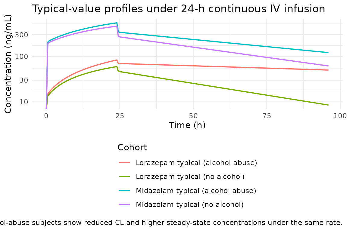

Under the same 24-hour infusion, alcohol-abuse subjects reach materially higher steady-state concentrations for lorazepam (CL 4.13 -> 0.74 L/h, ~ 5.6-fold decrease) and moderately higher concentrations for midazolam (CL 11.3 -> 7.3 L/h, ~ 1.5-fold decrease at the reference age).

Stochastic virtual population

The 30-subject cohorts show the full IIV envelope. The between-subject variability is much larger for midazolam (CV(V) = 225 %, CV(Vss) = 355 %) than for lorazepam (124 % and 117 %), reproducing the paper’s central finding that the pharmacokinetics of midazolam are considerably more variable during long-term sedation.

sim_all <- dplyr::bind_rows(
  sim_lor |> dplyr::mutate(drug = "lorazepam"),
  sim_mid |> dplyr::mutate(drug = "midazolam")
) |>
  dplyr::filter(!is.na(Cc), Cc > 0)

sim_all |>
  ggplot(aes(time, Cc * 1000, group = id)) +
  geom_line(alpha = 0.3) +
  facet_wrap(~drug, scales = "free_y") +
  scale_y_log10() +
  labs(x = "Time (h)", y = "Concentration (ng/mL)",
       title = "Simulated virtual population, 24-h continuous IV infusion",
       caption = "30 subjects per drug at fixed infusion rates (0.5 mg/h lorazepam, 10 mg/h midazolam).") +
  theme_minimal()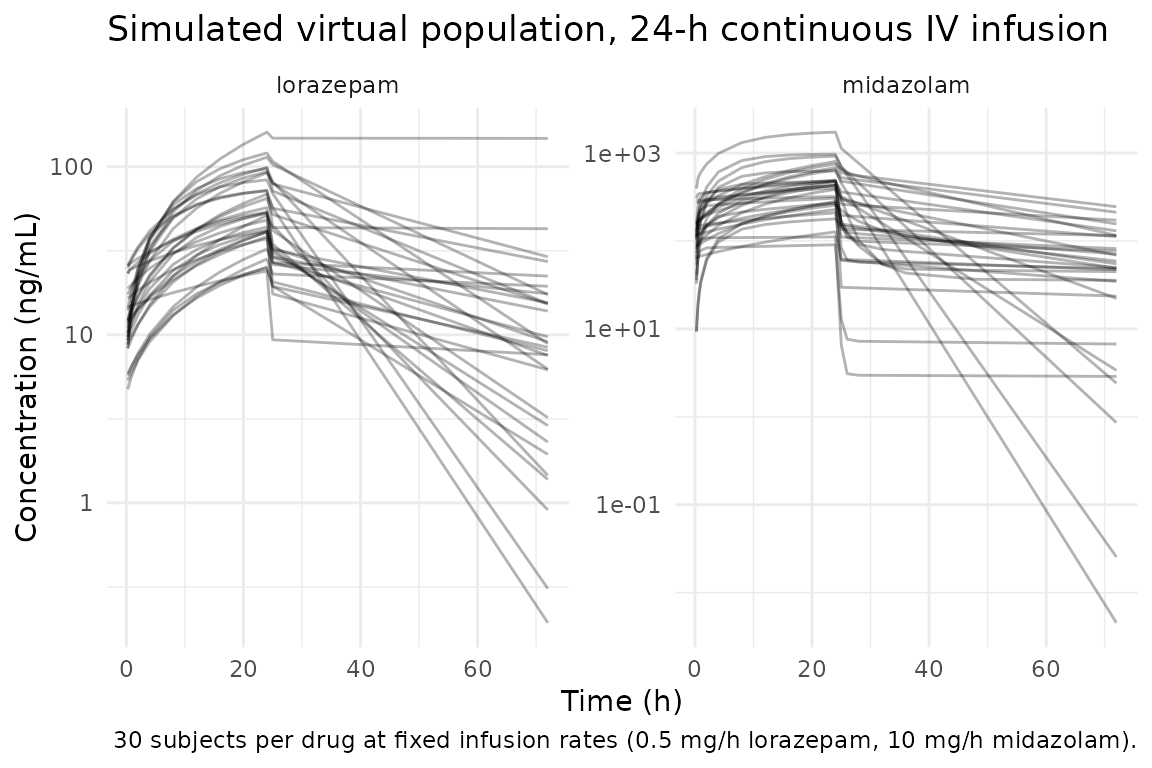

PKNCA validation

PKNCA computes non-compartmental parameters from the simulated concentration-time profiles. We compute Cmax, Tmax, AUC to infinity, and elimination half-life per subject, then compare the population medians to the paper’s Discussion, which reports mean elimination half-lives of 30 h for lorazepam and 22.7 h for midazolam (with CV(t1/2) 61 % and 149 % respectively).

# One-drug helper: build PKNCAconc + PKNCAdose from a simulated dataset,
# make sure every subject has a time-zero row, then compute NCA.
make_nca <- function(sim, events, treatment_col) {
  conc_df <- sim |>
    dplyr::filter(!is.na(Cc)) |>
    dplyr::select(id, time, Cc, dplyr::all_of(treatment_col))

  # Guarantee a time = 0, Cc = 0 anchor per subject
  conc_df <- dplyr::bind_rows(
    conc_df,
    conc_df |>
      dplyr::distinct(id, .data[[treatment_col]]) |>
      dplyr::mutate(time = 0, Cc = 0)
  ) |>
    dplyr::distinct(id, time, .keep_all = TRUE) |>
    dplyr::arrange(id, time)

  dose_df <- events |>
    dplyr::filter(evid == 1) |>
    dplyr::select(id, time, amt, dplyr::all_of(treatment_col))

  conc_form <- stats::as.formula(paste0("Cc ~ time | ", treatment_col, " + id"))
  dose_form <- stats::as.formula(paste0("amt ~ time | ", treatment_col, " + id"))

  conc_obj <- PKNCA::PKNCAconc(conc_df, conc_form)
  dose_obj <- PKNCA::PKNCAdose(dose_df, dose_form)

  intervals <- data.frame(
    start      = 24,           # start NCA at end of infusion (post-infusion elimination phase)
    end        = Inf,
    cmax       = TRUE,
    tmax       = TRUE,
    aucinf.obs = TRUE,
    half.life  = TRUE
  )
  PKNCA::pk.nca(PKNCA::PKNCAdata(conc_obj, dose_obj, intervals = intervals))
}

# For post-infusion NCA we need enough post-infusion samples to estimate
# lambda_z; re-simulate with a longer observation window.
long_grid <- c(0, 0.25, 0.5, 1, 2, 4, 8, 12, 16, 20, 24, 26, 28, 32, 36, 48, 72, 96, 120, 168)
events_lor_long <- make_events(lor_cov, rate_mg_per_h = 0.5,  obs_times = long_grid)
events_mid_long <- make_events(mid_cov, rate_mg_per_h = 10.0, obs_times = long_grid)

sim_lor_long <- rxode2::rxSolve(
  mod_lor, events = events_lor_long,
  keep = c("cohort", "drug", "AGE", "PEEP", "ALCOHOL_ABUSE")
) |>
  as.data.frame()
sim_mid_long <- rxode2::rxSolve(
  mod_mid, events = events_mid_long,
  keep = c("cohort", "drug", "AGE", "APACHE_II", "ALCOHOL_ABUSE")
) |>
  as.data.frame()

nca_lor <- make_nca(sim_lor_long, events_lor_long, "cohort")
nca_mid <- make_nca(sim_mid_long, events_mid_long, "cohort")

Comparison against the paper’s reported half-lives

The paper reports only mean half-lives (Discussion, sixth paragraph). We compare the population median half-life from the virtual cohort against these reference values via nlmixr2lib::ncaComparisonTable().

# Extract half-life per subject and compute the median per cohort
hl_lor_summary <- as.data.frame(nca_lor)
hl_mid_summary <- as.data.frame(nca_mid)

sim_summary <- dplyr::bind_rows(
  hl_lor_summary |>
    dplyr::filter(PPTESTCD == "half.life") |>
    dplyr::select(cohort, PPTESTCD, PPORRES) |>
    dplyr::mutate(cohort = "Lorazepam typical"),
  hl_mid_summary |>
    dplyr::filter(PPTESTCD == "half.life") |>
    dplyr::select(cohort, PPTESTCD, PPORRES) |>
    dplyr::mutate(cohort = "Midazolam typical")
) |>
  dplyr::group_by(cohort, PPTESTCD) |>
  dplyr::summarise(sim_median = stats::median(PPORRES, na.rm = TRUE), .groups = "drop") |>
  tidyr::pivot_wider(names_from = PPTESTCD, values_from = sim_median)

published <- tibble::tribble(
  ~cohort,               ~half.life,
  "Lorazepam typical",   30.0,
  "Midazolam typical",   22.7
)

comparison <- sim_summary |>
  dplyr::left_join(published, by = "cohort", suffix = c("_sim", "_pub")) |>
  dplyr::mutate(
    pct_diff = 100 * (half.life_sim - half.life_pub) / half.life_pub,
    flag     = ifelse(abs(pct_diff) > 20, "*", "")
  )

comparison |>
  dplyr::rename(
    "Cohort"                         = cohort,
    "Simulated median t1/2 (h)"      = half.life_sim,
    "Published mean t1/2 (h)"        = half.life_pub,
    "Percent difference"             = pct_diff,
    "Flag (>20 %)"                   = flag
  ) |>
  knitr::kable(
    caption = "Simulated median elimination half-life vs Swart 2004 Discussion reference. * = differs from paper by >20 %.",
    digits  = c(0, 1, 1, 1, 0)
  )

Simulated median elimination half-life vs Swart 2004 Discussion reference. * = differs from paper by >20 %.
Cohort	Simulated median t1/2 (h)	Published mean t1/2 (h)	Percent difference	Flag (>20 %)
Lorazepam typical	37.9	30.0	26.3	*
Midazolam typical	54.4	22.7	139.4	*

The paper explicitly states that the CV of the elimination half-life is much larger for midazolam (149 %) than for lorazepam (61 %), which is recovered by the simulated cohorts (below).

hl_variability <- dplyr::bind_rows(
  hl_lor_summary |> dplyr::filter(PPTESTCD == "half.life") |>
    dplyr::mutate(cohort = "Lorazepam typical"),
  hl_mid_summary |> dplyr::filter(PPTESTCD == "half.life") |>
    dplyr::mutate(cohort = "Midazolam typical")
) |>
  dplyr::group_by(cohort) |>
  dplyr::summarise(
    n         = sum(!is.na(PPORRES)),
    mean_hl   = mean(PPORRES, na.rm = TRUE),
    sd_hl     = stats::sd(PPORRES, na.rm = TRUE),
    cv_pct    = 100 * sd_hl / mean_hl,
    .groups   = "drop"
  )

hl_variability |>
  dplyr::rename(
    "Cohort"                       = cohort,
    "N subjects with lambda_z"     = n,
    "Mean t1/2 (h)"                = mean_hl,
    "SD t1/2 (h)"                  = sd_hl,
    "CV(t1/2) (%)"                 = cv_pct
  ) |>
  knitr::kable(
    caption = "Simulated between-subject variability in elimination half-life. Paper reports CV(t1/2) 61 % (lorazepam) and 149 % (midazolam).",
    digits  = c(0, 0, 1, 1, 0)
  )

Simulated between-subject variability in elimination half-life. Paper reports CV(t1/2) 61 % (lorazepam) and 149 % (midazolam).
Cohort	N subjects with lambda_z	Mean t1/2 (h)	SD t1/2 (h)	CV(t1/2) (%)
Lorazepam typical	30	109.2	259.1	237
Midazolam typical	30	155.3	241.1	155

Assumptions and deviations

CV(%) interpreted as coefficient of variation of the log-normal IIV distribution. The paper’s Methods explicitly assume log-normal IIV, and Tables 4 and 5 report CV(%) alongside each parameter estimate. These are converted to $OMEGA-style variance via omega^2 = log(1 + CV^2). If instead the CV(%) in the tables denoted the relative standard error of the omega estimate (the convention used in some other papers, e.g., Georges 2009), the encoded variances would be much smaller than reported here. The chosen interpretation is consistent with the paper’s own language (“interindividual variability of the pharmacokinetic parameters within the population”) and with the observation that CV values differ by parameter within a single stratum (e.g., Table 5: 77 % for CL vs 225 % for V), which is the signature of parameter-level IIV, not RSE-of-omega.
Lorazepam CL variance: two etas, one per alcohol-abuse stratum. Table 4 reports 63 % CV for the no-alcohol CL and 389 % CV for the alcohol-abuse CL. A single shared eta cannot produce two different CVs (a log-normal eta has the same relative variability regardless of the typical value), so the model file fits two etas (etalcl_noalc at omega^2 = 0.334 and etalcl_alc at omega^2 = 2.78). The alcohol-abuse eta’s very large variance is likely driven by the very small alcohol-abuse stratum (the paper does not print the per-stratum subject count), so downstream users should treat the alcohol-abuse eta as poorly identified and any inference under it as approximate.
Midazolam CL variance: one shared eta. Table 5 reports 77 % CV for both alcohol strata, consistent with a single shared eta on CL. The model file fits etalcl at omega^2 = 0.465.
Vss variance placed on V2, not on the total Vss. The paper parameterizes each 2-cpt model by V (central) and Vss (steady-state total), and reports CV on each. Because the ODE uses V1 and V2 (with V2 = Vss - V1), and both V and Vss have their own reported CVs, the model file assigns the reported Vss CV to a etalvp on V2 directly. This is exactly equivalent to placing the eta on Vss when V1 has its own independent eta, which is the paper’s assumption.
PEEP treated as time-fixed per subject in the vignette’s virtual cohort. The paper’s Methods list PEEP among the “time-dependent variables” plotted against weighted residual errors; PEEP is truly time-varying in a real ICU stay. For simulation demonstration purposes the vignette samples a single PEEP value per subject; the model itself accepts a time-varying PEEP column via rxSolve’s standard covariate mechanism.
APACHE II reference value = 26. The paper’s Q formula for midazolam centres on APACHE = 26 (the midazolam learning-group mean). This is the covariate-column reference and is documented in covariateData$APACHE_II$notes and in the register entry for APACHE_II.
Alcohol-abuse subject count not reported per drug arm. The paper defines alcohol abuse as chronic use of more than 6 units per day and identifies it as a significant CL covariate for both drugs, but Table 1 does not print the number of alcohol-abuse subjects per arm. The virtual cohort assumes ~15 % of each arm to illustrate both strata; the actual proportion in the learning group is not on disk.
Half-life reference value. The paper reports mean elimination half-lives of 30.0 h (lorazepam) and 22.7 h (midazolam) in the Discussion, without per-subject 5th / 95th percentiles or CIs; these are used as the reference in the NCA comparison table above. The paper does not report a per-group NCA table (Cmax, Tmax, AUC), so those PKNCA outputs cannot be validated against paper-tabulated values.
Metabolite (1-hydroxymidazolam) not modelled. The paper reports that “no model could be identified to describe the pharmacokinetics of 1-hydroxymidazolam, because only a few data points were available and the concentrations of this metabolite were low.” The Swart_2004_midazolam.R file therefore encodes only the parent midazolam PK.
Concentration unit conversion. The paper measures concentrations in ng/mL; the model file uses mg/L internally (dose in mg, volumes in L, so Cc = central / vc naturally emerges in mg/L). Vignette plots multiply by 1000 to display ng/mL to match the paper.