Valproic acid (Usman 2022)
Source:vignettes/articles/Usman_2022_valproic_acid.Rmd
Usman_2022_valproic_acid.RmdModel and source
- Citation: Usman M, Shaukat Q-u-A, Khokhar MI, Bilal R, Khan RR, Saeed HA, Ali M, Khan HM. Comparative pharmacokinetics of valproic acid among Pakistani and South Korean patients: A population pharmacokinetic study. PLoS One. 2022;17(8):e0272622. doi:10.1371/journal.pone.0272622. PMCID PMC9401156. Parameters from Table 2 and Eqs 1-4; covariate-model building from S1 Table (PsN scm output).
- Description: One-compartment population PK model with first-order elimination for intravenous valproic acid in adult Pakistani and South Korean patients, fitted to pooled routine therapeutic-drug-monitoring data (Usman 2022; 191 patients, 553 serum concentrations). Clearance carries a linear body-weight effect centred on the 67 kg pooled median and a multiplicative linear effect of the Pakistani centre (South Korean patients are the reference); volume of distribution carries a linear body-weight effect centred on 67 kg. Exponential IIV on CL and V, proportional residual error. Fitted in NONMEM 7.4.4 (ADVAN1 TRANS2, FOCE-I) with the covariate model built by PsN stepwise covariate modelling.
- Article: https://doi.org/10.1371/journal.pone.0272622 (open access)
- Supplement S1 Table (PsN stepwise covariate modelling output): https://doi.org/10.1371/journal.pone.0272622.s001
Population
Usman 2022 pooled routine therapeutic-drug-monitoring (TDM) data for intravenous valproic acid from two sources. The first is 92 Pakistani patients (218 samples) from Aziz Fatima Hospital, Faisalabad. The second is 99 South Korean patients (335 samples) from the earlier Park 2002 analysis (doi:10.1046/j.1365-2710.2002.00440.x). Together they give 191 patients and 553 serum concentrations, measured by ELISA at peak and trough.
The pooled cohort was 66.5% male, with median age 48 years (range 18-90) and median weight 67 kg (range 40-101). The Pakistani patients were heavier (median 71 kg, range 47-101) and older (median 54 years) than the Korean patients (median 60 kg, range 40-91; median 44 years). The median single dose was 1000 mg (range 500-1800 mg). Observed concentrations ranged from 3.38 to 106.4 mg/L (Usman 2022 Table 1). The paper does not state the indication, the infusion duration or the dosing interval.
The same information is available programmatically via
readModelDb("Usman_2022_valproic_acid")()$population.
Source trace
| Equation / parameter | Value | Source location |
|---|---|---|
| Structure: one compartment, IV input, first-order elimination | n/a | Results, ‘Population PK modelling’ (ADVAN1 TRANS2, FOCE-I) |
lcl (CL, South Korean, 67 kg) |
log(0.931) L/h | Table 2; Eqs 1 and 3 |
lvc (Vd, 67 kg) |
log(16.6) L | Table 2; Eq 4 |
e_nonkorean_cl (CL-CENT) |
0.386 | Table 2; Eqs 1-2; S1 Table ‘CLCENT-2’ |
e_wt_cl (CL-WT) |
0.0143 per kg | Table 2; Eq 3; S1 Table ‘CLWT-2’ |
e_wt_vc (Vd-WT) |
0.009 per kg | Table 2; Eq 4; S1 Table ‘VWT-2’ |
| Centring weight | 67 kg | Eqs 3-4 (‘67 is median body weight of pooled population’); Table 1 |
etalcl |
0.434^2 = 0.188356 | Table 2, ‘IIV CL (%)’ = 43.4 |
etalvc |
0.223^2 = 0.049729 | Table 2, ‘IIV Vd (%)’ = 22.3 |
propSd |
0.148 | Table 2, ‘Proportional Error’ |
CL equation:
cl = CL * (1 + 0.386 * (1 - RACE_KOREAN)) * (1 + 0.0143 * (WT - 67)) * exp(eta)
|
n/a | Eqs 1-3 with the PsN scm linear-relation code (see Errata) |
V equation:
vc = V * (1 + 0.009 * (WT - 67)) * exp(eta)
|
n/a | Eq 4 |
| Final covariate set (CL ~ CENT + WT, V ~ WT) | n/a | S1 Table, last backward step; Table 2 OFV 3344.6 = S1 Table 3344.60228 |
Typical values
The model is linear in each covariate, so the typical clearance and
volume for any patient can be written down from Table 2. The chunk below
solves the model with the random effects zeroed and checks that the
cl and vc columns match those hand
calculations. The check covers the reference patient (Korean, 67 kg) and
the median Pakistani (71 kg) and Korean (60 kg) patients.
mod <- readModelDb("Usman_2022_valproic_acid")
mod_typ <- rxode2::zeroRe(mod)
#> ℹ parameter labels from comments will be replaced by 'label()'

typ_cov <- tibble::tibble(
  id = 1:3,
  label = c("Reference (Korean, 67 kg)", "Median Pakistani (71 kg)", "Median Korean (60 kg)"),
  RACE_KOREAN = c(1, 0, 1),
  WT = c(67, 71, 60)
)
typ_ev <- typ_cov |>
  dplyr::select(id, RACE_KOREAN, WT) |>
  dplyr::cross_join(tibble::tibble(time = c(0, 1), evid = c(1L, 0L), amt = c(1000, 0))) |>
  dplyr::mutate(cmt = "central") |>
  dplyr::arrange(id, time)

typ_sim <- rxode2::rxSolve(mod_typ, events = typ_ev, returnType = "data.frame") |>
  dplyr::distinct(id, cl, vc)
#> ℹ omega/sigma items treated as zero: 'etalcl', 'etalvc'
#> Warning: multi-subject simulation without without 'omega'

typ <- typ_cov |>
  dplyr::left_join(typ_sim, by = "id") |>
  dplyr::mutate(
    cl_hand = 0.931 * (1 + 0.386 * (1 - RACE_KOREAN)) * (1 + 0.0143 * (WT - 67)),
    vc_hand = 16.6 * (1 + 0.009 * (WT - 67)),
    thalf_h = log(2) * vc / cl
  )

# cl and vc are algebraic, not integrated, so they agree to floating point.
stopifnot(
  max(abs(typ$cl / typ$cl_hand - 1)) < 1e-10,
  max(abs(typ$vc / typ$vc_hand - 1)) < 1e-10
)

typ |>
  dplyr::select(label, cl, vc, thalf_h) |>
  dplyr::rename(
    "Patient" = label,
    "Typical CL (L/h)" = cl,
    "Typical V (L)" = vc,
    "Half-life (h)" = thalf_h
  ) |>
knitr::kable(digits = 3)| Patient | Typical CL (L/h) | Typical V (L) | Half-life (h) |
|---|---|---|---|
| Reference (Korean, 67 kg) | 0.931 | 16.600 | 12.359 |
| Median Pakistani (71 kg) | 1.364 | 17.198 | 8.738 |
| Median Korean (60 kg) | 0.838 | 15.554 | 12.869 |
At 67 kg the Pakistani typical clearance is 0.931 x 1.386 = 1.290 L/h. The paper’s Eq 2 prints it as 0.931 + 0.386 = 1.317 L/h. The two differ by 2%; the Errata section explains why the multiplicative form is used.
Virtual cohort
Original observed data are not publicly available. The cohort below has two arms of 150 patients, one per centre. Body weights are drawn log-normally around each centre’s median (71 kg Pakistani, 60 kg Korean) and truncated to the observed range of that centre (Table 1). Each patient receives 1000 mg (the Table 1 median single dose) as a 1-hour intravenous infusion. The paper does not report the infusion duration; one hour is the labelled rate for intravenous valproate.
# rxSetSeed() fixes rxode2's draw for a given solver thread count, not across
# thread counts, so every assertion below is on a centre or a robust quantile.
set.seed(20220824)
rxode2::rxSetSeed(20220824)

n_per_arm <- 150

draw_weight <- function(n, median_wt, lo, hi, sdlog) {
  wt <- exp(rnorm(n * 3, log(median_wt), sdlog))
  wt <- wt[wt >= lo & wt <= hi]
  wt[seq_len(n)]
}

cohort <- dplyr::bind_rows(
  tibble::tibble(
    id = seq_len(n_per_arm),
    population = "Pakistani",
    RACE_KOREAN = 0,
    WT = draw_weight(n_per_arm, 71, 47, 101, 0.15)
  ),
  tibble::tibble(
    id = n_per_arm + seq_len(n_per_arm),
    population = "South Korean",
    RACE_KOREAN = 1,
    WT = draw_weight(n_per_arm, 60, 40, 91, 0.165)
  )
)
stopifnot(!anyNA(cohort$WT), !anyDuplicated(cohort$id))

cohort |>
  dplyr::group_by(population) |>
  dplyr::summarise(
    N = dplyr::n(),
    `Median WT (kg)` = median(WT),
    `Min WT (kg)` = min(WT),
    `Max WT (kg)` = max(WT),
    .groups = "drop"
  ) |>
  dplyr::rename("Population" = population) |>
knitr::kable(digits = 1)| Population | N | Median WT (kg) | Min WT (kg) | Max WT (kg) |
|---|---|---|---|---|
| Pakistani | 150 | 69.7 | 48.2 | 93.8 |
| South Korean | 150 | 59.5 | 41.1 | 89.7 |
Single-dose simulation and PKNCA
A single 1000 mg dose, sampled densely to 120 h, gives each patient a full profile. PKNCA’s AUC0-inf and half-life are then compared with the closed-form one-compartment values for the same patient: AUC = dose / CL and t1/2 = ln 2 x V / CL. Both sides use the same drawn parameters, so this check tests the solve and the NCA set-up, not the cohort.
obs_times <- sort(unique(c(0, 0.5, 1, 1.5, 2, 3, 4, 6, 8, 12, 16, 24, 36, 48, 72, 96, 120)))

sd_ev <- dplyr::bind_rows(
  cohort |> dplyr::mutate(time = 0, evid = 1L, amt = 1000, rate = 1000),
  cohort |>
    dplyr::cross_join(tibble::tibble(time = obs_times)) |>
    dplyr::mutate(evid = 0L, amt = 0, rate = 0)
) |>
  dplyr::mutate(cmt = "central") |>
  dplyr::arrange(id, time, dplyr::desc(evid))

sd_sim <- rxode2::rxSolve(
  mod,
  events = sd_ev,
  keep = c("population", "WT"),
  rtol = 1e-10,
  atol = 1e-12,
  returnType = "data.frame"
)
#> ℹ parameter labels from comments will be replaced by 'label()'
stopifnot(!anyNA(sd_sim$Cc))
# Floor the integrator's sub-atol undershoot before NCA (none expected here,
# but the floor keeps the log-down trapezoid finite if one appears).
stopifnot(all(sd_sim$Cc >= -1e-6 * max(sd_sim$Cc)))

# IPRED: the comparison is against the closed form, so no residual error.
conc_df <- sd_sim |>
  dplyr::filter(!is.na(Cc)) |>
  dplyr::mutate(Cc = pmax(Cc, 0)) |>
  dplyr::select(id, time, Cc, population)

conc_df <- dplyr::bind_rows(
  conc_df,
  conc_df |> dplyr::distinct(id, population) |> dplyr::mutate(time = 0, Cc = 0)
) |>
  dplyr::distinct(id, population, time, .keep_all = TRUE) |>
  dplyr::arrange(id, time)

dose_df <- cohort |>
  dplyr::transmute(id, population, time = 0, amt = 1000)

conc_obj <- PKNCA::PKNCAconc(conc_df, Cc ~ time | population + id)
dose_obj <- PKNCA::PKNCAdose(dose_df, amt ~ time | population + id, duration = 1)
intervals <- data.frame(
  start = 0,
  end = Inf,
  cmax = TRUE,
  tmax = TRUE,
  aucinf.obs = TRUE,
  half.life = TRUE
)
nca_res <- PKNCA::pk.nca(PKNCA::PKNCAdata(conc_obj, dose_obj, intervals = intervals))
par_by_id <- sd_sim |>
  dplyr::distinct(id, population, cl, vc) |>
  dplyr::mutate(
    kel = cl / vc,
    aucinf.obs = 1000 / cl,
    half.life = log(2) / kel,
    # End-of-infusion concentration of a 1 h zero-order input.
    cmax = (1000 / 1) / cl * (1 - exp(-kel * 1))
  )

nca_wide <- as.data.frame(nca_res) |>
  dplyr::filter(PPTESTCD %in% c("cmax", "aucinf.obs", "half.life")) |>
  dplyr::select(id, population, PPTESTCD, PPORRES) |>
  tidyr::pivot_wider(names_from = PPTESTCD, values_from = PPORRES)

ident <- nca_wide |>
  dplyr::left_join(par_by_id, by = c("id", "population"), suffix = c("_nca", "_cf")) |>
  dplyr::mutate(
    pct_auc = 100 * (aucinf.obs_nca / aucinf.obs_cf - 1),
    pct_thalf = 100 * (half.life_nca / half.life_cf - 1),
    pct_cmax = 100 * (cmax_nca / cmax_cf - 1)
  )

# Same parameters on both sides: the only differences are trapezoid error on
# the 1 h infusion and the terminal-phase point selection. Cmax is sampled
# exactly at the end of infusion, so it matches to integrator precision.
stopifnot(
  abs(median(ident$pct_auc)) < 2,
  quantile(abs(ident$pct_auc), 0.9) < 5,
  abs(median(ident$pct_thalf)) < 2,
  quantile(abs(ident$pct_thalf), 0.9) < 5,
  max(abs(ident$pct_cmax)) < 1e-4
)

reference <- par_by_id |>
  dplyr::group_by(population) |>
  dplyr::summarise(
    cmax = median(cmax),
    aucinf.obs = median(aucinf.obs),
    half.life = median(half.life),
    .groups = "drop"
  )

cmp <- ncaComparisonTable(
  nca_res,
  reference,
  by = "population",
  params = c("cmax", "aucinf.obs", "half.life"),
  units = c(cmax = "mg/L", aucinf.obs = "mg*h/L", half.life = "h")
)
cmp |>
  dplyr::rename("Population" = population) |>
knitr::kable(caption = "Median PKNCA result vs median closed-form one-compartment value, single 1000 mg dose infused over 1 h.")| NCA parameter | Population | Reference | Simulated | % diff |
|---|---|---|---|---|
| Cmax (mg/L) | Pakistani | 54.6 | 54.6 | +0.0% |
| Cmax (mg/L) | South Korean | 62.2 | 62.2 | -0.0% |
| AUC0-∞ (obs) (mg*h/L) | Pakistani | 828 | 828 | -0.0% |
| AUC0-∞ (obs) (mg*h/L) | South Korean | 1220 | 1220 | -0.0% |
| t½ (h) | Pakistani | 9.76 | 9.76 | -0.0% |
| t½ (h) | South Korean | 12.6 | 12.6 | -0.0% |
The paper reports no NCA, so the reference column here is the closed form from the model’s own parameters. None of the rows is starred, so none differs by more than 20%.
Replicate Figure 1: CL and Vd by population
Usman 2022 Figure 1 is a pair of box plots of the individual CL and Vd in the two populations. The Results text gives their medians (ranges): CL 1.21 (0.55-2.96) L/h Pakistani and 0.97 (0.39-3.38) L/h Korean; Vd 17.6 (10.4-27.5) L Pakistani and 15.2 (8.36-25.1) L Korean.
indiv <- sd_sim |>
  dplyr::distinct(id, population, cl, vc) |>
  tidyr::pivot_longer(c(cl, vc), names_to = "parameter", values_to = "value") |>
  dplyr::mutate(parameter = dplyr::recode(parameter, cl = "CL (L/h)", vc = "Vd (L)"))

ggplot(indiv, aes(population, value)) +
  geom_boxplot() +
  facet_wrap(~parameter, scales = "free_y") +
  labs(
    x = NULL,
    y = NULL,
    title = "Individual CL and Vd by population",
    caption = "Replicates Figure 1 of Usman 2022 with the simulated virtual cohort."
  )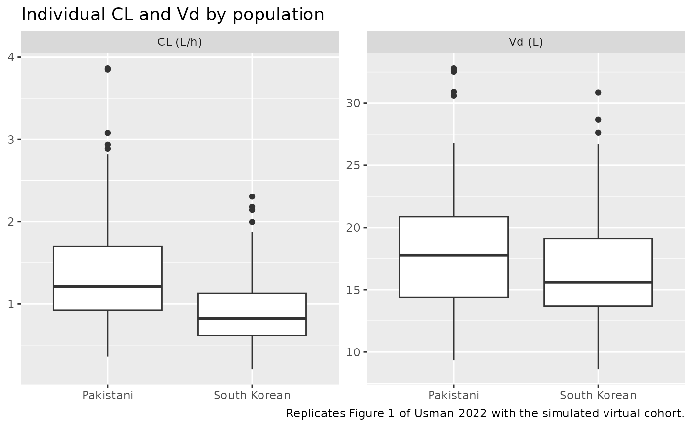
fig1_ref <- tibble::tribble(
  ~population,    ~parameter, ~published,
  "Pakistani",    "CL (L/h)", 1.21,
  "South Korean", "CL (L/h)", 0.97,
  "Pakistani",    "Vd (L)",   17.6,
  "South Korean", "Vd (L)",   15.2
)

fig1_cmp <- indiv |>
  dplyr::group_by(population, parameter) |>
  dplyr::summarise(simulated = median(value), .groups = "drop") |>
  dplyr::left_join(fig1_ref, by = c("population", "parameter")) |>
  dplyr::mutate(pct_diff = 100 * (simulated / published - 1))

fig1_cmp |>
  dplyr::rename(
    "Population" = population,
    "Parameter" = parameter,
    "Simulated median" = simulated,
    "Published median" = published,
    "% diff" = pct_diff
  ) |>
knitr::kable(digits = 2)| Population | Parameter | Simulated median | Published median | % diff |
|---|---|---|---|---|
| Pakistani | CL (L/h) | 1.21 | 1.21 | -0.15 |
| Pakistani | Vd (L) | 17.78 | 17.60 | 1.05 |
| South Korean | CL (L/h) | 0.82 | 0.97 | -15.65 |
| South Korean | Vd (L) | 15.60 | 15.20 | 2.65 |
# Vd: the model reproduces the published medians. A 10% band admits the
# cohort-median spread (median of 150 log-normal draws with 22% IIV moves by
# about 2%) and still fails on a mis-transcribed volume or weight slope.
fig1_v <- dplyr::filter(fig1_cmp, parameter == "Vd (L)")
stopifnot(max(abs(fig1_v$pct_diff)) < 10)

# CL: recorded deviation, not gated (see the text below and the Errata).
fig1_cl <- dplyr::filter(fig1_cmp, parameter == "CL (L/h)")
stopifnot(
  fig1_cl$simulated[fig1_cl$population == "Pakistani"] >
    fig1_cl$simulated[fig1_cl$population == "South Korean"]
)
The volume medians agree with the published ones. The clearance medians do not. At the centre median weights the model’s typical clearance is 1.364 L/h for a Pakistani patient (+13% against 1.21 L/h) and 0.838 L/h for a Korean patient (-14% against 0.97 L/h). The ratio is 1.63, which is 1.386 for the centre effect times 1.175 for the weight difference. The Figure 1 medians give 1.21 / 0.97 = 1.25. The simulated cohort medians in the table scatter around the typical values, because CL has 43% IIV, so one of them can land near a published median by chance. The ratio is the comparison that does not depend on the draw. Table 2 and Eqs 1-3 cannot give a ratio as small as 1.25: the weight effect alone already gives 1.175.
Figure 1 is therefore more likely drawn from individual estimates that do not come from the final model, for example from a model without the centre effect, where shrinkage pulls the two centres together. The paper does not say which model Figure 1 comes from. The packaged model follows Table 2. The ordering, with Pakistani clearance higher, matches the paper’s conclusion, and that is the only thing the chunk above gates for clearance.
Repeated dosing against the observed concentration range
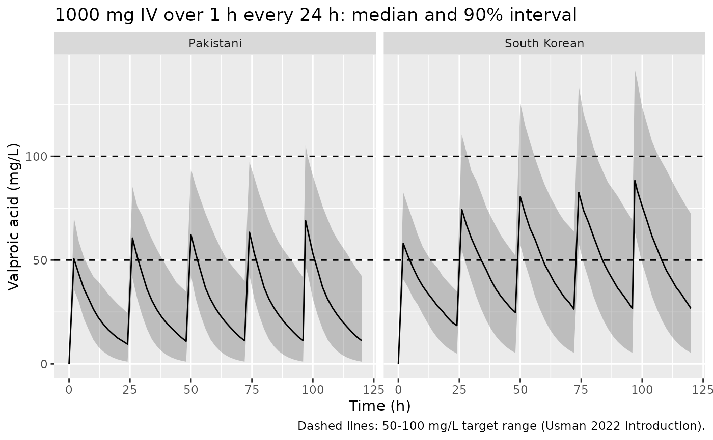
The paper does not report the dosing interval. The Methods give a daily dose of 500-1600 mg, and the Table 1 median single dose (1000 mg) equals the median of that daily range, which suggests once-daily dosing. The simulation below gives 1000 mg over 1 h every 24 h for 5 days. It shows peak (end of infusion) and trough concentrations on day 5, with residual error, against the 3.38-106.4 mg/L range observed in the pooled data and the 50-100 mg/L target range quoted in the paper’s Introduction.
tau <- 24
n_dose <- 5
md_ev <- dplyr::bind_rows(
  cohort |>
    dplyr::cross_join(tibble::tibble(time = tau * (seq_len(n_dose) - 1))) |>
    dplyr::mutate(evid = 1L, amt = 1000, rate = 1000),
  cohort |>
    dplyr::cross_join(tibble::tibble(time = c(0, seq(0, tau * n_dose, by = 2), tau * (n_dose - 1) + 1))) |>
    dplyr::mutate(evid = 0L, amt = 0, rate = 0)
) |>
  dplyr::mutate(cmt = "central") |>
  dplyr::distinct(id, time, evid, .keep_all = TRUE) |>
  dplyr::arrange(id, time, dplyr::desc(evid))

md_sim <- rxode2::rxSolve(mod, events = md_ev, keep = "population", returnType = "data.frame")
stopifnot(!anyNA(md_sim$Cc))

md_sim |>
  dplyr::group_by(population, time) |>
  dplyr::summarise(
    Q05 = quantile(Cc, 0.05),
    Q50 = median(Cc),
    Q95 = quantile(Cc, 0.95),
    .groups = "drop"
  ) |>
  ggplot(aes(time, Q50)) +
  geom_ribbon(aes(ymin = Q05, ymax = Q95), alpha = 0.25) +
  geom_line() +
  geom_hline(yintercept = c(50, 100), linetype = "dashed") +
  facet_wrap(~population) +
  labs(
    x = "Time (h)",
    y = "Valproic acid (mg/L)",
    title = "1000 mg IV over 1 h every 24 h: median and 90% interval",
    caption = "Dashed lines: 50-100 mg/L target range (Usman 2022 Introduction)."
  )
day5 <- md_sim |>
  dplyr::filter(time %in% c(tau * (n_dose - 1) + 1, tau * n_dose)) |>
  dplyr::mutate(sample = ifelse(time == tau * n_dose, "Trough", "Peak (end of infusion)"))

day5_sum <- day5 |>
  dplyr::group_by(population, sample) |>
  dplyr::summarise(
    `Median (mg/L)` = median(sim),
    `5th pct (mg/L)` = quantile(sim, 0.05),
    `95th pct (mg/L)` = quantile(sim, 0.95),
    `% inside 3.38-106.4 mg/L` = 100 * mean(sim >= 3.38 & sim <= 106.4),
    .groups = "drop"
  )
day5_sum |>
  dplyr::rename("Population" = population, "Sample" = sample) |>
knitr::kable(digits = 1)| Population | Sample | Median (mg/L) | 5th pct (mg/L) | 95th pct (mg/L) | % inside 3.38-106.4 mg/L |
|---|---|---|---|---|---|
| Pakistani | Peak (end of infusion) | 67.4 | 43.1 | 105.0 | 96.0 |
| Pakistani | Trough | 11.5 | 1.0 | 43.1 | 81.3 |
| South Korean | Peak (end of infusion) | 87.8 | 54.6 | 144.3 | 74.7 |
| South Korean | Trough | 26.0 | 4.8 | 72.0 | 94.7 |
# The medians of both peak and trough sit inside the observed range in both
# populations; a mis-scaled volume or clearance moves them out by multiples.
stopifnot(all(day5_sum$`Median (mg/L)` > 3.38 & day5_sum$`Median (mg/L)` < 106.4))
On this regimen the upper tail of the Korean peaks lies above the highest concentration observed in the pooled data. The observed samples come from doses of 500-1800 mg under unreported regimens, so the table describes one plausible regimen rather than the study’s own dosing.
Assumptions and deviations
-
Centre effect is multiplicative (Eqs 1-2). The
paper’s Eq 2 prints the Pakistani clearance as
CL = (0.931 + 0.386) = 1.317. The covariate model was built with PsN stepwise covariate modelling. S1 Table names the retained relationsCLCENT-2,CLWT-2andVWT-2, which is PsN’s linear relation. For a categorical covariate PsN writes that relation asIF(CENT.EQ.0) CLCENT = 1 ; Most commonandIF(CENT.EQ.1) CLCENT = (1 + THETA), then multiplies the typical CL by it. Eq 1 reproduces that code, including its ‘Most common’ comment, with 0.931 written in place of 1. The packaged model therefore uses the fitted form, CL = 0.931 x (1 + 0.386 x CENT) x (1 + 0.0143 x (WT - 67)). This gives a Pakistani clearance at 67 kg of 1.290 L/h instead of the printed 1.317 L/h, a 2% difference. -
Covariate encoding. CENT (0 = South Korean, 1 =
Pakistani) is encoded through the existing
RACE_KOREANindicator as CENT = 1 - RACE_KOREAN. In this dataset the centre and the ethnicity coincide. For a patient who is neither Korean nor Pakistani the model extrapolates, andRACE_KOREAN = 0then applies the Pakistani clearance. - Age is not in the final model. The text under Eq 4 says that Eq 4 gives the influence of ‘body weight and age’ on Vd. Eq 4 and Table 2 carry only body weight. S1 Table shows that V-AGE entered in the last forward step and was removed in the backward step (dOFV 6.19 < 6.63). The final OFV in S1 Table (3344.60) equals the one in Table 2 (3344.6).
- Separate eta on V. Eq 4 writes the volume random effect as eta1, the same symbol as the clearance random effect in Eq 3. Table 2 reports separate IIV for CL and Vd and no correlation, so the model has two independent etas.
- IIV scale. Table 2 gives IIV as a percentage, with RSE on the variance scale. The bootstrap 95% CI half-width divided by (1.96 x estimate x RSE) is 0.51 for CL and 0.50 for Vd. This is the 0.5 expected when the percentage is 100 x sqrt(omega). The log-normal CV reading, omega = log(1 + CV^2), predicts 0.54 for CL. Omega is therefore (IIV/100)^2.
-
Residual error is an SD. The Table 2 rows run CL,
Vd, Proportional Error, then the three scm covariate coefficients. This
is the NONMEM THETA order, with PsN appending covariate thetas after the
base model’s. Proportional Error is therefore THETA(3), the SD
multiplying EPS with SIGMA fixed at 1, so
propSd = 0.148. - Figure 1 clearance medians not reproduced. See the Figure 1 section: the published medians imply a much smaller between-centre clearance ratio than Table 2 gives. The Vd medians are reproduced.
- Dosing used in the simulations. The infusion duration (1 h used) and the dosing interval (24 h used) are not reported. Neither affects the model parameters; they only shape the illustrative simulations.
- Text inconsistency. The Methods mention comparing ‘Vd and CL of vancomycin’ between the centres; the drug throughout is valproic acid.
- Literature check. A search of Europe PMC on 2026-10-05 found no erratum or correction for this article.