Metronidazole (Cohen-Wolkowiez 2012)
Source:vignettes/articles/CohenWolkowiez_2012_metronidazole.Rmd
CohenWolkowiez_2012_metronidazole.RmdModel and source
- Citation: Cohen-Wolkowiez M, Ouellet D, Smith PB, et al. Population pharmacokinetics of metronidazole evaluated using scavenged samples from preterm infants. Antimicrob Agents Chemother. 2012;56(4):1828-1837. doi:10.1128/AAC.06071-11
- Description: One-compartment IV population PK model for metronidazole in preterm infants (Cohen-Wolkowiez 2012). Clearance scales linearly with body weight (reference 1.5 kg) and as a power function of postmenstrual age (reference 32 weeks); central volume scales linearly with body weight.
- Article: https://doi.org/10.1128/AAC.06071-11
Population
The model was built from a 5-center prospective open-label PK study (the Antimicrobial PK in High-Risk Infants trial, sponsored by the Pediatric Pharmacology Research Unit). Thirty-three subjects were enrolled and 32 were included in the analysis after one subject was excluded for during-infusion-only sampling; one further subject was excluded from the PK data set due to outlier-related issues, leaving 32 subjects with 116 plasma metronidazole concentrations used in the model build. Cohort demographics (Cohen-Wolkowiez 2012 Tables 1 and 2):
- Gestational age at birth: median 27 weeks (range 22-32).
- Postnatal age: median 41 days (range 0-97).
- Postmenstrual age: median 32 weeks (range 24-43).
- Weight: median 1495 g (range 678-3850 g).
- Sex: 17 of 32 (53 percent) female.
- Race: 16 of 32 (50 percent) White; 4 of 32 (9 percent recorded as Hispanic ethnicity).
- Serum creatinine: median 0.5 mg/dL (range 0.1-4.7).
- Metronidazole dose: median 8 mg/kg (range 4-15) given as an intravenous infusion at clinician-prescribed intervals (median 12 h, range 5.9-48 h).
Of the 116 concentrations used in the analysis, 104 (90 percent) were
scavenged from discarded clinical specimens and 12 were obtained from
study-specific timed blood draws. The same information is available
programmatically via the model’s population metadata
(readModelDb("CohenWolkowiez_2012_metronidazole")$population).
Source trace
The per-parameter origin is recorded as an in-file comment next to
each ini() entry in
inst/modeldb/specificDrugs/CohenWolkowiez_2012_metronidazole.R.
The table below collects them in one place for review.
| Equation / parameter | Value | Source location |
|---|---|---|
| Structural model: 1-compartment IV | n/a | Results, “Population PK model building”; Table 3 final-model row |
lcl = log(0.0397) (theta_CL, L/h) |
0.0397 | Table 4, “CL (liters/h)” (RSE 10.9 percent) |
lvc = log(1.07) (theta_V, L) |
1.07 | Table 4, “V (liters)” (RSE 15.0 percent) |
e_wt_cl = fixed(1) |
1 | Table 3 final-model row: linear (wt/1.5) scaling;
estimated body-size exponent excluded for lack of fit improvement
(Results) |
e_wt_vc = fixed(1) |
1 | Table 3 final-model row: linear (wt/1.5) scaling on
V |
e_page_cl = 2.49 (theta_CL-PMA) |
2.49 | Table 4, “CL,PMA” (RSE 29.8 percent) |
etalcl variance 0.16608 |
omega^2 = log(1 + 0.425^2) | Table 4, “Interindividual variance CL (CV%) = 42.5” (RSE 28.5 percent) |
propSd = 0.135 |
13.5 CV percent | Table 4, “Residual variance (CV%) Blood draws sigma_1^2 = 13.5” (RSE 24.5 percent) |
d/dt(central) = -kel * central |
n/a | Results, “Population PK model building”: 1-compartment model |
Concentration Cc = central / vc
|
n/a | 1-compartment IV; observation is plasma metronidazole concentration |
Virtual cohort
Original observed concentrations are not publicly available. The simulations below use virtual cohorts whose covariate distributions approximate the published trial demographics. We build one cohort per PMA stratum, matching the published BGA-group structure in Table 2.
set.seed(1128)

# Helper: build one cohort as a self-contained event table.
# - dose_mg_per_kg sets the maintenance dose; loading_mg_per_kg sets the
#   first-dose loading amount (set to NA for no loading dose).
# - tau_h is the dosing interval used by the PMA-based regimen.
# - WT (kg) and PAGE (months) are drawn from a per-stratum truncated
#   uniform on the published PMA week range; weight covers each
#   stratum's reported weight range.
# - id_offset shifts subject IDs so multiple cohorts stay disjoint.
make_cohort <- function(n, pma_week_lo, pma_week_hi,
                        wt_kg_lo, wt_kg_hi,
                        dose_mg_per_kg, loading_mg_per_kg,
                        tau_h, n_doses, obs_every_h,
                        treatment, id_offset = 0L) {
  ids <- id_offset + seq_len(n)
  wt   <- runif(n, wt_kg_lo, wt_kg_hi)
  pma_weeks <- runif(n, pma_week_lo, pma_week_hi)
  page <- pma_weeks / 4.35

  subj <- tibble::tibble(
    id        = ids,
    WT        = wt,
    PAGE      = page,
    treatment = treatment
  )

  loading_amt <- subj$WT * loading_mg_per_kg
  maint_amt   <- subj$WT * dose_mg_per_kg

  load_rows <- tibble::tibble(
    id        = subj$id,
    time      = 0,
    amt       = loading_amt,
    evid      = 1L,
    cmt       = "central",
    WT        = subj$WT,
    PAGE      = subj$PAGE,
    treatment = subj$treatment
  )

  maint_times <- seq(tau_h, by = tau_h, length.out = n_doses - 1L)
  maint_rows <- tibble::tibble(
    id        = rep(subj$id, each = length(maint_times)),
    time      = rep(maint_times, times = n),
    amt       = rep(maint_amt,   each = length(maint_times)),
    evid      = 1L,
    cmt       = "central",
    WT        = rep(subj$WT,  each = length(maint_times)),
    PAGE      = rep(subj$PAGE, each = length(maint_times)),
    treatment = rep(subj$treatment, each = length(maint_times))
  )

  end_time <- tau_h * n_doses
  obs_times <- seq(0, end_time, by = obs_every_h)
  obs_rows <- tibble::tibble(
    id        = rep(subj$id, each = length(obs_times)),
    time      = rep(obs_times, times = n),
    amt       = NA_real_,
    evid      = 0L,
    cmt       = "central",
    WT        = rep(subj$WT,  each = length(obs_times)),
    PAGE      = rep(subj$PAGE, each = length(obs_times)),
    treatment = rep(subj$treatment, each = length(obs_times))
  )

  dplyr::bind_rows(load_rows, maint_rows, obs_rows) |>
    dplyr::arrange(id, time, dplyr::desc(evid)) |>
    as.data.frame()
}

# Published PMA-based dosing regimen (Cohen-Wolkowiez 2012 Table 1):
# 15 mg/kg loading, then 7.5 mg/kg every 12 h (PMA < 34 wk) / 8 h (34-40 wk) / 6 h (> 40 wk).
events <- dplyr::bind_rows(
  make_cohort(n = 100, pma_week_lo = 24, pma_week_hi = 29,
              wt_kg_lo = 0.7, wt_kg_hi = 1.5,
              dose_mg_per_kg = 7.5, loading_mg_per_kg = 15,
              tau_h = 12, n_doses = 14L, obs_every_h = 1,
              treatment = "PMA < 34 wk (q12h)", id_offset =   0L),
  make_cohort(n = 100, pma_week_lo = 30, pma_week_hi = 33,
              wt_kg_lo = 1.2, wt_kg_hi = 2.5,
              dose_mg_per_kg = 7.5, loading_mg_per_kg = 15,
              tau_h = 12, n_doses = 14L, obs_every_h = 1,
              treatment = "PMA < 34 wk (q12h)", id_offset = 100L),
  make_cohort(n = 100, pma_week_lo = 34, pma_week_hi = 40,
              wt_kg_lo = 1.8, wt_kg_hi = 3.5,
              dose_mg_per_kg = 7.5, loading_mg_per_kg = 15,
              tau_h = 8,  n_doses = 21L, obs_every_h = 1,
              treatment = "PMA 34-40 wk (q8h)", id_offset = 200L),
  make_cohort(n = 100, pma_week_lo = 41, pma_week_hi = 43,
              wt_kg_lo = 2.5, wt_kg_hi = 3.9,
              dose_mg_per_kg = 7.5, loading_mg_per_kg = 15,
              tau_h = 6,  n_doses = 29L, obs_every_h = 1,
              treatment = "PMA > 40 wk (q6h)", id_offset = 300L)
)

stopifnot(!anyDuplicated(unique(events[, c("id", "time", "evid")])))
Simulation
mod <- readModelDb("CohenWolkowiez_2012_metronidazole")

sim <- rxode2::rxSolve(
  mod,
  events = events,
  keep   = c("treatment", "WT", "PAGE")
) |>
  as.data.frame() |>
  dplyr::filter(time > 0)
#> ℹ parameter labels from comments will be replaced by 'label()'
Replicate published figures
Figure 7-style simulated time-concentration profiles in typical subjects
Cohen-Wolkowiez 2012 Figure 7 shows simulated time-concentration
profiles for four typical subjects (PMA 26, 32, 36, 41 weeks; weights
900, 1900, 2800, 3800 g) receiving the proposed PMA-based dosing
regimen. We reproduce the figure with rxode2::zeroRe() to
remove between-subject variability:
mod_typical <- mod |> rxode2::zeroRe()
#> ℹ parameter labels from comments will be replaced by 'label()'

typical_specs <- tibble::tibble(
  treatment = c("PMA 26 wk, 900 g",
                "PMA 32 wk, 1900 g",
                "PMA 36 wk, 2800 g",
                "PMA 41 wk, 3800 g"),
  pma_weeks = c(26, 32, 36, 41),
  wt_kg     = c(0.9, 1.9, 2.8, 3.8),
  tau_h     = c(12,  12,  8,   6),
  n_doses   = c(14L, 14L, 21L, 29L)
)

build_typical <- function(spec) {
  page <- spec$pma_weeks / 4.35
  load_amt  <- spec$wt_kg * 15
  maint_amt <- spec$wt_kg * 7.5
  maint_times <- seq(spec$tau_h, by = spec$tau_h, length.out = spec$n_doses - 1L)
  obs_times   <- seq(0, spec$tau_h * spec$n_doses, by = 0.25)
  data.frame(
    id        = 1L,
    time      = c(0, maint_times, obs_times),
    amt       = c(load_amt, rep(maint_amt, length(maint_times)),
                  rep(NA_real_, length(obs_times))),
    evid      = c(1L, rep(1L, length(maint_times)),
                  rep(0L, length(obs_times))),
    cmt       = "central",
    WT        = spec$wt_kg,
    PAGE      = page,
    treatment = spec$treatment
  )
}

typical_events <- do.call(rbind, lapply(seq_len(nrow(typical_specs)),
                                        function(i) build_typical(typical_specs[i, ])))

sim_typical <- rxode2::rxSolve(
  mod_typical,
  events = typical_events,
  keep   = c("treatment")
) |>
  as.data.frame() |>
  dplyr::filter(time > 0)
#> ℹ omega/sigma items treated as zero: 'etalcl'

ggplot(sim_typical, aes(time, Cc)) +
  geom_line() +
  geom_hline(yintercept = 8, linetype = "dashed", colour = "grey40") +
  facet_wrap(~ factor(treatment, levels = typical_specs$treatment), scales = "free_x") +
  labs(x = "Time (h)", y = "Metronidazole concentration (mg/L)",
       caption = "Replicates Figure 7 of Cohen-Wolkowiez 2012; dashed line is the MIC=8 mg/L target.")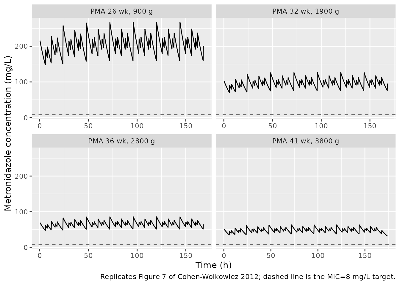
VPC of the PMA-based regimen
sim |>
  dplyr::group_by(time, treatment) |>
  dplyr::summarise(
    Q05 = quantile(Cc, 0.05, na.rm = TRUE),
    Q50 = quantile(Cc, 0.50, na.rm = TRUE),
    Q95 = quantile(Cc, 0.95, na.rm = TRUE),
    .groups = "drop"
  ) |>
  ggplot(aes(time, Q50)) +
  geom_ribbon(aes(ymin = Q05, ymax = Q95), alpha = 0.25) +
  geom_line() +
  geom_hline(yintercept = 8, linetype = "dashed", colour = "grey40") +
  facet_wrap(~ treatment, scales = "free_x") +
  labs(x = "Time (h)", y = "Metronidazole concentration (mg/L)",
       caption = "Stochastic simulation (100 subjects per stratum, eta on CL) of the proposed PMA-based regimen; dashed line is the MIC=8 mg/L target.")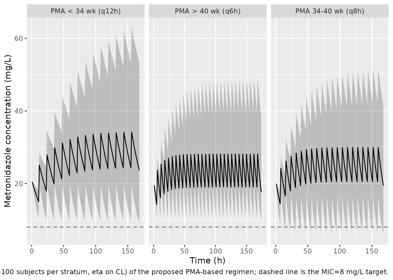
PKNCA validation
PKNCA is used to compute Cmax, Cmin, AUC over the last dosing interval, and apparent half-life on the simulated cohort. The terminal dosing interval is selected per treatment so steady state is approached.
last_interval <- sim |>
  dplyr::group_by(treatment) |>
  dplyr::summarise(
    end_time = max(time),
    tau      = dplyr::case_when(
      treatment[1] == "PMA < 34 wk (q12h)" ~ 12,
      treatment[1] == "PMA 34-40 wk (q8h)" ~ 8,
      treatment[1] == "PMA > 40 wk (q6h)"  ~ 6
    ),
    .groups = "drop"
  ) |>
  dplyr::mutate(
    start_ss = end_time - tau,
    end_ss   = end_time
  )

sim_nca <- sim |>
  dplyr::filter(!is.na(Cc)) |>
  dplyr::select(id, time, Cc, treatment) |>
  as.data.frame()

dose_df <- events |>
  dplyr::filter(evid == 1) |>
  dplyr::select(id, time, amt, treatment) |>
  as.data.frame()

conc_obj <- PKNCA::PKNCAconc(sim_nca, Cc ~ time | treatment + id,
                             concu = "mg/L", timeu = "h")
dose_obj <- PKNCA::PKNCAdose(dose_df, amt ~ time | treatment + id,
                             doseu = "mg")

# Steady-state interval per treatment (last dosing interval).
intervals_ss <- dose_df |>
  dplyr::group_by(treatment, id) |>
  dplyr::summarise(start = max(time), .groups = "drop") |>
  dplyr::left_join(last_interval |> dplyr::select(treatment, tau),
                   by = "treatment") |>
  dplyr::mutate(end = start + tau,
                cmax = TRUE, cmin = TRUE,
                auclast = TRUE, cav = TRUE) |>
  dplyr::select(-tau) |>
  as.data.frame()

# Terminal half-life on the post-final-dose decay phase.
intervals_thalf <- dose_df |>
  dplyr::group_by(treatment, id) |>
  dplyr::summarise(start = max(time), .groups = "drop") |>
  dplyr::mutate(end = Inf, half.life = TRUE) |>
  as.data.frame()

intervals <- dplyr::bind_rows(intervals_ss, intervals_thalf) |>
  dplyr::mutate(
    cmax      = !is.na(cmax)      & cmax,
    cmin      = !is.na(cmin)      & cmin,
    auclast   = !is.na(auclast)   & auclast,
    cav       = !is.na(cav)       & cav,
    half.life = !is.na(half.life) & half.life
  )

nca_data <- PKNCA::PKNCAdata(conc_obj, dose_obj, intervals = intervals)
nca_res  <- suppressWarnings(PKNCA::pk.nca(nca_data))

res_tbl <- as.data.frame(nca_res$result)
Comparison against published half-life (Table 5)
Cohen-Wolkowiez 2012 Table 5 reports median individual empirical Bayesian half-life by gestational-age-at-birth group: 20.5 h (less-than 26 weeks), 18.6 h (26-29 weeks), 16.7 h (30-32 weeks), 19.1 h overall. The simulated half-life from the packaged model is below; differences are driven by the BGA-to-PMA mapping in the virtual cohorts and by the different stratification axis (PMA vs BGA), so a one-to-one match is not expected.
half_life_simulated <- res_tbl |>
  dplyr::filter(PPTESTCD == "half.life") |>
  dplyr::group_by(treatment) |>
  dplyr::summarise(
    median_thalf_h = median(PPORRES, na.rm = TRUE),
    q05_thalf_h    = quantile(PPORRES, 0.05, na.rm = TRUE),
    q95_thalf_h    = quantile(PPORRES, 0.95, na.rm = TRUE),
    .groups = "drop"
  )

knitr::kable(half_life_simulated, digits = 2,
caption = "Simulated terminal half-life by PMA stratum (median, 5th, 95th percentile across 100 virtual subjects per stratum). Published reference: Table 5 of Cohen-Wolkowiez 2012 reports 16.7-20.5 h across BGA strata.")| treatment | median_thalf_h | q05_thalf_h | q95_thalf_h |
|---|---|---|---|
| PMA 34-40 wk (q8h) | 12.84 | 5.46 | 24.47 |
| PMA < 34 wk (q12h) | 22.68 | 10.83 | 49.74 |
| PMA > 40 wk (q6h) | 8.87 | 5.47 | 17.15 |
Steady-state Cmax / Cmin / Cavg by PMA stratum
ss_nca <- res_tbl |>
  dplyr::filter(PPTESTCD %in% c("cmax", "cmin", "auclast", "cav")) |>
  dplyr::group_by(treatment, PPTESTCD) |>
  dplyr::summarise(
    median = median(PPORRES, na.rm = TRUE),
    q05    = quantile(PPORRES, 0.05, na.rm = TRUE),
    q95    = quantile(PPORRES, 0.95, na.rm = TRUE),
    .groups = "drop"
  ) |>
  dplyr::mutate(PPTESTCD = factor(PPTESTCD, levels = c("cmax", "cmin", "cav", "auclast")))

knitr::kable(ss_nca, digits = 2,
caption = "Simulated steady-state NCA parameters (Cmax, Cmin, Cavg, AUClast) over the last dosing interval. Units: concentrations in mg/L; AUC in mg*h/L.")| treatment | PPTESTCD | median | q05 | q95 |
|---|---|---|---|---|
| PMA 34-40 wk (q8h) | auclast | 194.69 | 82.77 | 368.78 |
| PMA 34-40 wk (q8h) | cav | 24.34 | 10.35 | 46.10 |
| PMA 34-40 wk (q8h) | cmax | 29.97 | 16.48 | 51.52 |
| PMA 34-40 wk (q8h) | cmin | 19.46 | 5.97 | 41.07 |
| PMA < 34 wk (q12h) | auclast | 342.84 | 164.32 | 694.98 |
| PMA < 34 wk (q12h) | cav | 28.57 | 13.69 | 57.92 |
| PMA < 34 wk (q12h) | cmax | 34.13 | 19.62 | 62.89 |
| PMA < 34 wk (q12h) | cmin | 23.65 | 9.10 | 53.21 |
| PMA > 40 wk (q6h) | auclast | 134.60 | 83.04 | 260.01 |
| PMA > 40 wk (q6h) | cav | 22.43 | 13.84 | 43.34 |
| PMA > 40 wk (q6h) | cmax | 28.10 | 19.76 | 48.80 |
| PMA > 40 wk (q6h) | cmin | 17.58 | 9.24 | 38.29 |
Predicted steady-state trough concentrations (cmin) at
the proposed PMA-based regimen are well above the MIC=8 mg/L target
across strata, consistent with the paper’s reported greater-than-90
percent target attainment in simulated subjects (Figure 5C and Figure
6).
Assumptions and deviations
-
Scavenged-sample bias term omitted. The published
final model (Cohen-Wolkowiez 2012 Table 4) reports a multiplicative
scavenged- sample bias factor
theta_SCAV = 0.713(95 percent CI 0.581-0.899), representing a 30 percent underestimation of metronidazole concentrations in scavenged versus blood-draw samples, plus an elevated proportional residual error for scavenged samples (29.0 CV percent vs 13.5 CV percent for blood draws). These are artifacts of the scavenged sampling design (delayed centrifugation, uncertain documentation, sample-handling variability) rather than features of the underlying drug PK. The packaged model retains only the blood-draw residual error (propSd = 0.135) so that simulations represent the true drug concentration time-course; downstream users who explicitly want to simulate a scavenged-sample mixture can applytheta_SCAV * Ccand the elevated 29 percent CV residual outside the packaged model. The omitted parameters are recorded incovariatesDataExcluded$SCAVof the model file. -
Univariable serum-creatinine effect omitted.
Cohen-Wolkowiez 2012 Table 3 reports a
(0.5/SCR)^theta_CL_SCReffect on CL in the univariable step (OFV drop 14.3), but the final multivariable model excluded it because (i) the association was driven by a single outlier with SCR=4.7 mg/dL, and (ii) SCR is strongly correlated with PMA in preterm infants and did not improve fit beyond PMA. The packaged model follows the published final model and excludes SCR. - PNA / BGA covariate effects omitted. Both were screened univariably and excluded from the final model in favor of PMA.
-
PMA versus PAGE units. The paper uses postmenstrual
age in weeks with a 32-week reference; the nlmixr2lib canonical
covariate
PAGEis in months. The model reparameterises internally as(PAGE * 4.35 / 32)^theta_CL_PMAso the published 32-week reference is preserved without changing the canonical covariate unit. -
Allometric body-size scaling. Both CL and V scale
linearly with body weight at the reference 1.5 kg (Cohen-Wolkowiez 2012
Table 3:
theta * (wt/1.5)). An estimated body-size exponent was tested by the authors but excluded for lack of improvement; the packaged model encodes these asfixed(1)exponents so the fixed status is visible inini(). - No IIV on V. After body weight was incorporated as a covariate for V, the V-IIV nonparametric estimate was close to zero and the parameter was excluded from the final model. The packaged model follows that decision and carries IIV on CL only.
- Race / ethnicity distribution. The published cohort was 50 percent White with 9 percent Hispanic ethnicity; the model does not carry a race covariate, so race-balanced virtual cohorts are not required for the simulations above.
- PMA strata in virtual cohorts. Paper Table 5 stratifies by birth-gestational-age (BGA) group, but the model uses PMA as the CL-maturation covariate; the validation virtual cohorts above are stratified by PMA (matching the proposed dosing-regimen strata in Table 1) rather than by BGA, so the half-life comparison is qualitative.