Guselkumab PPPASI (Iwaki 2021)
Source:vignettes/articles/Iwaki_2021_guselkumab.Rmd
Iwaki_2021_guselkumab.Rmd
library(nlmixr2lib)
library(rxode2)
#> rxode2 5.1.8 using 2 threads (see ?getRxThreads)
#>   no cache: create with `rxCreateCache()`
library(dplyr)
#>
#> Attaching package: 'dplyr'
#> The following objects are masked from 'package:stats':
#>
#>     filter, lag
#> The following objects are masked from 'package:base':
#>
#>     intersect, setdiff, setequal, union
library(tidyr)
library(ggplot2)
library(PKNCA)
#>
#> Attaching package: 'PKNCA'
#> The following object is masked from 'package:stats':
#>
#>     filter
Model and source
- Citation: Iwaki Y, Shibata S, Hu C. Pharmacokinetic/Pharmacodynamic Analysis of Guselkumab for Treatment of Palmoplantar Pustulosis: Clinical Implications of Guselkumab Dose, Disease Severity, and Smoking in Japanese Patients. J Clin Pharmacol. 2022;62(2):182-189. doi:10.1002/jcph.1953. PK structure and parameters taken from Yao Z et al. J Clin Pharmacol. 2018;58(5):613-627. doi:10.1002/jcph.1063; see modellib(‘Yao_2018_guselkumab’).
- Description: PK/PD model for guselkumab (anti-IL-23 p19 human IgG1-lambda mAb) and the Palmoplantar Pustulosis Area and Severity Index (PPPASI) in Japanese adults with palmoplantar pustulosis (Iwaki 2021). PK: the one-compartment model with first-order SC absorption of Yao 2018, applied unchanged. PD: the PPPASI score is a bounded outcome score analysed as an ordered categorical variable (721 categories of 0.1 points) whose probabilities are intervals of a beta distribution with mean mu and precision tau; logit(mu) = logit(baseline) - placebo effect - drug effect + linear disease progression, where the placebo effect is Pmax * (1 - exp(-kp * t)) and the drug effect is Emax * (1 - R), with R a type I indirect-response latent variable inhibited by serum guselkumab (IC50 fixed at 1e-6 ug/mL).
- Article: https://doi.org/10.1002/jcph.1953
- PK model: https://doi.org/10.1002/jcph.1063 (Yao 2018; packaged as
Yao_2018_guselkumab)
Iwaki 2021 describes the longitudinal Palmoplantar Pustulosis Area and Severity Index (PPPASI) in Japanese patients with palmoplantar pustulosis (PPP) treated with guselkumab or placebo. The analysis was sequential: the population PK model of Yao 2018, developed in plaque psoriasis, was applied to the PPP patients to obtain individual PK parameters, and those were then held fixed while the PK/PD model was estimated. Iwaki 2021 reports no PK estimates of its own, so the PK layer of this model is the Yao 2018 model unchanged (one compartment, first-order SC absorption, body weight on CL/F and V/F, diabetes and race on CL/F).
The PD layer follows the bounded-outcome-score approach of Hu et
al. for the PASI score. The PPPASI score (0 to 72 in 0.1-point steps) is
mapped to k / 720 with k = 0, ..., 720 and
treated as an ordered categorical variable with
where B is the CDF of a beta distribution with mean
mu and precision tau (shape parameters
mu * tau and (1 - mu) * tau). The mean is
with a type I indirect-response latent variable
Population
The analysis pooled a phase 2 proof-of-concept study (49 patients randomized 1:1 to guselkumab 200 mg or placebo SC at weeks 0 and 4, efficacy through week 24) and a phase 3 confirmatory study (159 patients randomized 1:1:1 to guselkumab 100 mg, 200 mg or placebo SC at weeks 0, 4 and 12 and then every 8 weeks, efficacy through week 52; the placebo group was rerandomized 1:1 to 100 or 200 mg at weeks 16 and 20, then every 8 weeks). Both were double-blind, placebo-controlled trials at multiple sites in Japan.
The PK/PD dataset held 207 patients, all Japanese, with 160 women (77%) and 125 smokers (60%). Median baseline body weight was 59.7 kg (range 37.0 to 98.2) and median baseline PPPASI was 24.6 (range 4.8 to 59.4); 1813 PK and 2718 PPPASI observations were analysed (Iwaki 2021 Methods, “Clinical Study Designs”, and Results, “Exploratory Assessments of the Observed Data”). Age is not reported. The same information is available programmatically:
readModelDb("Iwaki_2021_guselkumab")()$population[c(
  "n_subjects", "n_studies", "weight_median", "sex_female_pct",
  "race_ethnicity", "smoker_pct", "baseline_pppasi"
)]
#> $n_subjects
#> [1] 207
#>
#> $n_studies
#> [1] 2
#>
#> $weight_median
#> [1] 59.7
#>
#> $sex_female_pct
#> [1] 77.3
#>
#> $race_ethnicity
#> [1] "All Asian (Japanese)"
#>
#> $smoker_pct
#> [1] 60.4
#>
#> $baseline_pppasi
#> [1] "median 24.6 (range 4.8-59.4) on the 0-72 scale"
Source trace
Each ini() value carries an in-file comment naming its
source. They are collected here.
| Equation / parameter | Value | Source location |
|---|---|---|
lcl (CL/F) |
log(0.516 L/day) | Yao 2018 Table 4 (final reduced model) |
lvc (V/F) |
log(13.5 L) | Yao 2018 Table 4 |
lka (ka) |
log(1.11 1/day) | Yao 2018 Table 4 |
e_wt_cl, e_wt_vc
|
0.998, 0.829 | Yao 2018 Table 4 footnotes b and c |
e_diab_cl, e_race_cl
|
1.12, 1.11 | Yao 2018 Table 4 footnote b |
etalcl + etalvc, etalka
|
0.126736, 0.083133, 0.078400; 1.6641 | Yao 2018 Table 4 (IIV 35.6%, 28.0%, 129%; correlation 0.834) |
propSd, addSd
|
0.200, 0.00289 ug/mL (fixed) | Yao 2018 Table 4 |
| PK structure and covariates | n/a | Iwaki 2021 Methods, “Population PK Modeling” |
ltau (PhiBeta) |
log(64.7) | Iwaki 2021 Table 1; Supplemental THETA(1)
|
logitrbase (mu_b) |
logit(0.356) | Iwaki 2021 Table 1; Supplemental THETA(2)
|
lpmax (Fp, Pmax) |
log(1.55) | Iwaki 2021 Table 1; Supplemental THETA(3)
|
lkpbo (kp) |
log(0.004 1/day) | Iwaki 2021 Table 1; Supplemental THETA(4)
|
lkout (kout) |
log(0.00139 1/day) | Iwaki 2021 Table 1; Supplemental THETA(5)
|
lic50 (IC50) |
log(1e-6 ug/mL), fixed | Iwaki 2021 Table 1 and Results; Supplemental THETA(6)
FIX |
lemax (DE) |
log(2.97) | Iwaki 2021 Table 1; Supplemental THETA(7)
|
dp_slope (kdspg) |
0.000944 1/day | Iwaki 2021 Table 1; Supplemental THETA(8)
|
etalogitrbase |
0.507 (normal, logit scale) | Iwaki 2021 Table 1; Methods |
etalkpbo, etalkout,
etalemax
|
1.69, 1.04, 0.320 (log-normal) | Iwaki 2021 Table 1 |
etadp_slope |
10.3 (proportional: kdspg * (1 + eta)) | Iwaki 2021 Table 1; Methods; Supplemental
DSPG = THETA(8) * (1 + ETA(5))
|
| Beta-CDF ordered-categorical likelihood | n/a | Iwaki 2021 Methods, “Population PK/PD Modeling”; Supplemental
$ERROR
|
logit(mu) equation |
n/a | Iwaki 2021 Methods; Supplemental $ERROR (signs from the
code, see Errata) |
d/dt(latent_pppasi),
latent_pppasi(0) <- 1
|
n/a | Iwaki 2021 Methods; Supplemental $DES and
A_0(3) = 1
|
Virtual cohort
The observed data are not public. The cohort below follows the phase
3 design, the larger and longer of the two studies: guselkumab 100 mg or
200 mg at weeks 0, 4 and 12 and then every 8 weeks, and placebo at weeks
0, 4 and 12 followed by guselkumab 100 or 200 mg at weeks 16 and 20 and
then every 8 weeks, through week 52. Body weight is log-normal around
the cohort median of 59.7 kg, truncated to the observed range; every
subject is non-White (RACE_WHITE = 0) and non-diabetic
(DIS_DIAB = 0, see Assumptions).
rxode2::rxSetSeed(20211)
set.seed(20211)

n_per_arm <- 150L
wk <- 7

active_weeks <- c(0, 4, 12, 20, 28, 36, 44)
switch_weeks <- c(16, 20, 28, 36, 44)
arms <- tibble(
  treatment = c("Gus 100 mg", "Gus 200 mg", "Placebo -> Gus 100 mg", "Placebo -> Gus 200 mg"),
  dose_mg = c(100, 200, 100, 200),
  dose_weeks = list(active_weeks, active_weeks, switch_weeks, switch_weeks)
)

# Weekly grid for the score, plus a daily grid over the last dosing interval
# (weeks 44 to 52) for the steady-state NCA.
obs_times <- sort(unique(c(seq(0, 52 * wk, by = wk), seq(44 * wk, 52 * wk, by = 1))))

make_arm <- function(i, id_offset) {
  arm <- arms[i, ]
  ids <- id_offset + seq_len(n_per_arm)
  wt <- exp(rnorm(n_per_arm, log(59.7), 0.2))
  wt <- pmin(pmax(wt, 37.0), 98.2)
  covs <- tibble(id = ids, WT = wt, DIS_DIAB = 0L, RACE_WHITE = 0L)
  doses <- tidyr::expand_grid(id = ids, time = arm$dose_weeks[[1]] * wk) |>
    mutate(amt = arm$dose_mg, cmt = "depot", evid = 1L, dvid = NA_integer_)
  obs <- tidyr::expand_grid(id = ids, time = obs_times) |>
    mutate(amt = 0, cmt = NA_character_, evid = 0L, dvid = 1L)
  bind_rows(doses, obs) |>
    left_join(covs, by = "id") |>
    mutate(treatment = arm$treatment)
}

events <- bind_rows(lapply(seq_len(nrow(arms)), function(i) {
  make_arm(i, id_offset = (i - 1L) * n_per_arm)
})) |>
  arrange(id, time, desc(evid))

stopifnot(!anyDuplicated(unique(events[, c("id", "time", "evid")])))
Simulation
rxSolve() returns the beta mean mu_pppasi
and the shape parameters alpha_pppasi and
beta_pppasi for every subject and visit. A PPPASI score is
drawn from the ordered categorical distribution by drawing
x from the beta distribution and taking
k = floor(721 * x), which falls in category k
with exactly the probability B((k + 1)/721) - B(k/721) of
the model. Given mu, visits are independent, as in the
source model.
mod <- readModelDb("Iwaki_2021_guselkumab")
sim <- rxode2::rxSolve(mod, events = events, keep = c("treatment", "WT")) |>
  as.data.frame()
#> ℹ parameter labels from comments will be replaced by 'label()'

sim <- sim |>
  mutate(
    pppasi = floor(721 * rbeta(n(), alpha_pppasi, beta_pppasi)) / 10,
    week = time / wk
  )

score <- sim |>
  filter(week == round(week)) |>
  group_by(id) |>
  mutate(
    pppasi_bl = pppasi[week == 0],
    cfb = pppasi - pppasi_bl,
    pct_improve = 100 * (pppasi_bl - pppasi) / pppasi_bl
  ) |>
  ungroup()
Replicate published figures
PPPASI change from baseline by arm (cf. Figure 2)
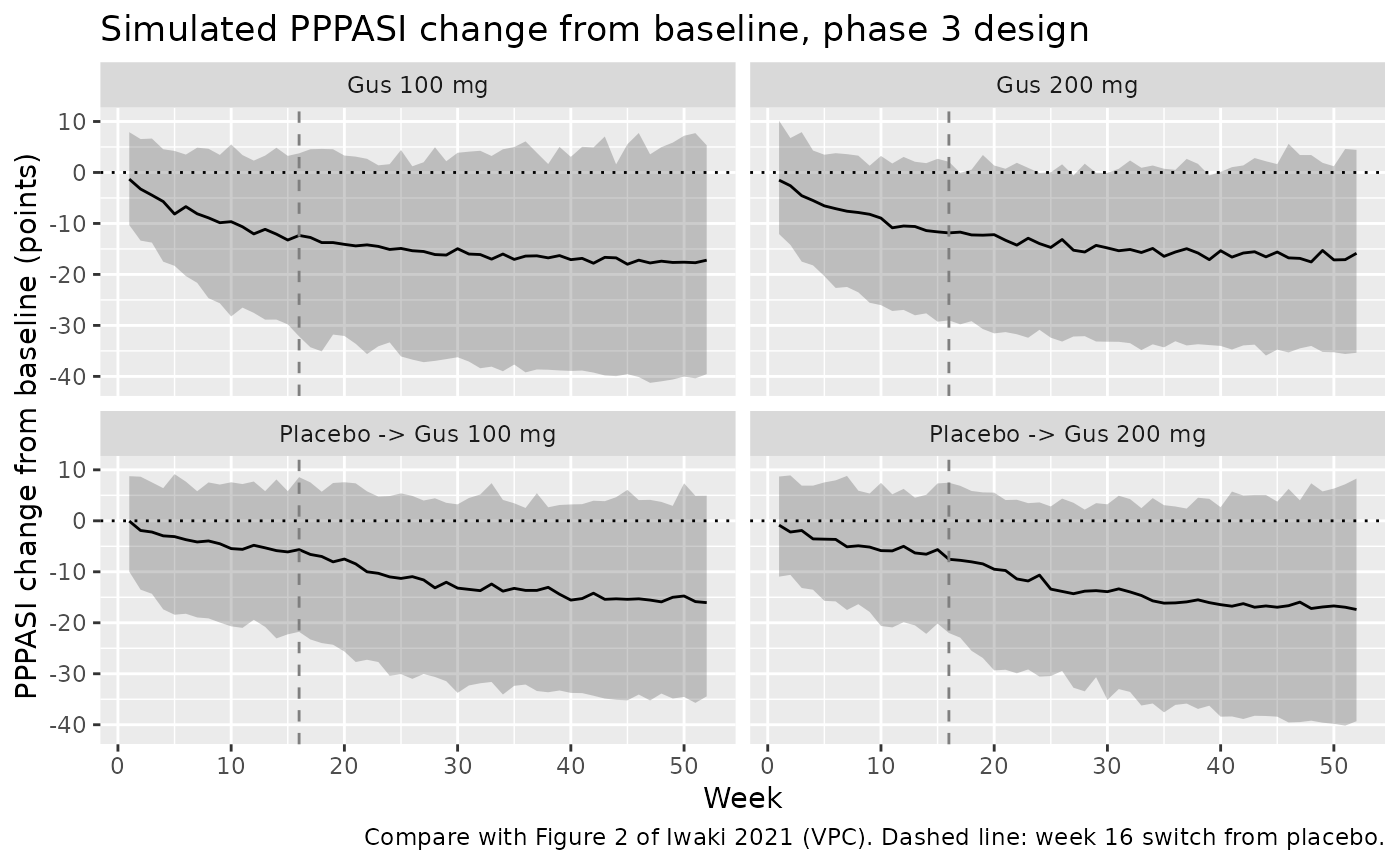
Figure 2 of Iwaki 2021 is a VPC of the change from baseline of the PPPASI score by study and treatment group. The simulated median and 90% prediction interval for the phase 3 design are shown below.
score |>
  filter(week > 0) |>
  group_by(treatment, week) |>
  summarise(
    Q05 = quantile(cfb, 0.05),
    Q50 = quantile(cfb, 0.50),
    Q95 = quantile(cfb, 0.95),
    .groups = "drop"
  ) |>
  ggplot(aes(week, Q50)) +
  geom_ribbon(aes(ymin = Q05, ymax = Q95), alpha = 0.25) +
  geom_line() +
  geom_hline(yintercept = 0, linetype = "dotted") +
  geom_vline(xintercept = 16, linetype = "dashed", colour = "grey50") +
  facet_wrap(~treatment) +
  labs(
    x = "Week", y = "PPPASI change from baseline (points)",
    title = "Simulated PPPASI change from baseline, phase 3 design",
    caption = "Compare with Figure 2 of Iwaki 2021 (VPC). Dashed line: week 16 switch from placebo."
  )
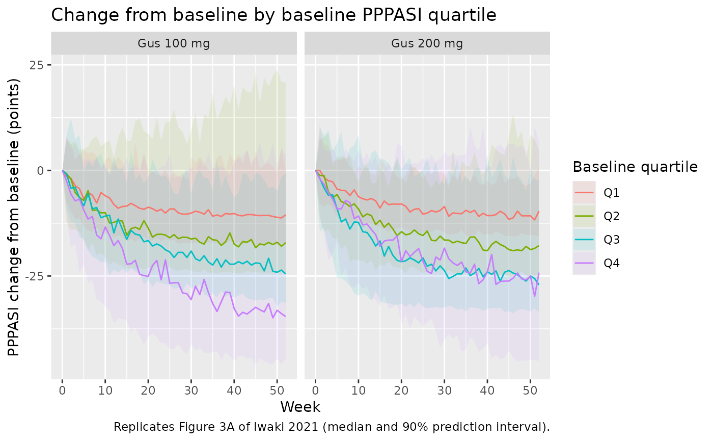
Change from baseline by baseline-severity quartile (Figure 3A)
bl_q <- score |>
  filter(week == 0, treatment %in% c("Gus 100 mg", "Gus 200 mg")) |>
  group_by(treatment) |>
  mutate(bl_quartile = paste0("Q", dplyr::ntile(pppasi_bl, 4))) |>
  ungroup() |>
  select(id, bl_quartile)

score_q <- score |>
  inner_join(bl_q, by = "id")

score_q |>
  group_by(treatment, bl_quartile, week) |>
  summarise(
    Q05 = quantile(cfb, 0.05),
    Q50 = quantile(cfb, 0.50),
    Q95 = quantile(cfb, 0.95),
    .groups = "drop"
  ) |>
  ggplot(aes(week, Q50, colour = bl_quartile, fill = bl_quartile)) +
  geom_ribbon(aes(ymin = Q05, ymax = Q95), alpha = 0.10, colour = NA) +
  geom_line() +
  facet_wrap(~treatment) +
  labs(
    x = "Week", y = "PPPASI change from baseline (points)",
    colour = "Baseline quartile", fill = "Baseline quartile",
    title = "Change from baseline by baseline PPPASI quartile",
    caption = "Replicates Figure 3A of Iwaki 2021 (median and 90% prediction interval)."
  )
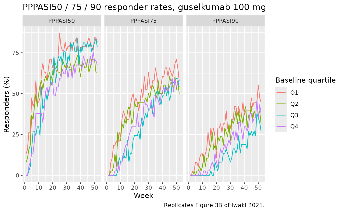
Responder rates with 100 mg by baseline quartile (Figure 3B)
resp <- score_q |>
  filter(treatment == "Gus 100 mg", week > 0) |>
  group_by(bl_quartile, week) |>
  summarise(
    PPPASI50 = mean(pct_improve >= 50),
    PPPASI75 = mean(pct_improve >= 75),
    PPPASI90 = mean(pct_improve >= 90),
    .groups = "drop"
  ) |>
  pivot_longer(starts_with("PPPASI"), names_to = "endpoint", values_to = "rate")

ggplot(resp, aes(week, 100 * rate, colour = bl_quartile)) +
  geom_line() +
  facet_wrap(~endpoint) +
  labs(
    x = "Week", y = "Responders (%)", colour = "Baseline quartile",
    title = "PPPASI50 / 75 / 90 responder rates, guselkumab 100 mg",
    caption = "Replicates Figure 3B of Iwaki 2021."
  )
Checks against the paper’s statements
The paper reports its PD results graphically, so the checks below test the statements it makes in the text.
Baseline. The typical baseline on the 0-1 scale is 0.356, i.e. about 25.6 points, against an observed median baseline of 24.6.
bl <- score |> filter(week == 0)
median(bl$pppasi)
#> [1] 25.7
stopifnot(abs(median(bl$pppasi) - 24.6) < 3)
100 mg and 200 mg are almost identical. With IC50
fixed at 1e-6 ug/mL, Cp / (IC50 + Cp) is 1 for any
measurable concentration, so the drug effect does not depend on dose.
The typical-value predictions for the two doses coincide; the
deterministic difference in the predicted mean score is negligible.
mod_typ <- rxode2::zeroRe(mod)
#> ℹ parameter labels from comments will be replaced by 'label()'
typ_events <- events |>
  filter(id %in% c(1L, n_per_arm + 1L)) |>
  mutate(WT = 59.7)
typ <- rxode2::rxSolve(mod_typ, events = typ_events, keep = "treatment") |>
  as.data.frame() |>
  mutate(score_mean = 72 * mu_pppasi) |>
  select(treatment, time, score_mean) |>
  pivot_wider(names_from = treatment, values_from = score_mean)
#> ℹ omega/sigma items treated as zero: 'etalcl', 'etalvc', 'etalka', 'etalogitrbase', 'etalkpbo', 'etalkout', 'etalemax', 'etadp_slope'
#> Warning: multi-subject simulation without without 'omega'
max_diff <- max(abs(typ[["Gus 100 mg"]] - typ[["Gus 200 mg"]]))
max_diff
#> [1] 8.381268e-07
stopifnot(max_diff < 0.01)
Larger absolute but similar relative improvement at higher baseline. Figure 3A shows larger reductions in absolute points for patients with a higher baseline score, while Figure 3B shows similar responder rates across baseline quartiles.
wk52 <- score_q |>
  filter(treatment == "Gus 100 mg", week == 52) |>
  group_by(bl_quartile) |>
  summarise(
    median_cfb = median(cfb),
    PPPASI50 = mean(pct_improve >= 50),
    .groups = "drop"
  )
knitr::kable(wk52, digits = 2, caption = "Week 52, guselkumab 100 mg, by baseline quartile.")| bl_quartile | median_cfb | PPPASI50 |
|---|---|---|
| Q1 | -10.5 | 0.82 |
| Q2 | -17.1 | 0.63 |
| Q3 | -24.5 | 0.78 |
| Q4 | -34.6 | 0.68 |
q1 <- wk52$median_cfb[wk52$bl_quartile == "Q1"]
q4 <- wk52$median_cfb[wk52$bl_quartile == "Q4"]
# Absolute reductions differ several-fold between the extreme quartiles
# (Q4 roughly 3x Q1 here); the bound only requires Q4 to be the larger.
stopifnot(q4 < q1 - 5)
Placebo response and worsening. The placebo effect lowers the score through week 16, and the disease-progression term, whose between-subject variance is large, lets some placebo patients worsen.
PKNCA validation
Iwaki 2021 gives one PK reference point: the IC50 sensitivity analysis fixed IC50 at 1 ug/mL, “around the trough concentration of guselkumab under the 100-mg regimen”. The steady-state NCA over the final dosing interval (weeks 44 to 52) is compared against that value for the 100 mg arm.
sim_nca <- sim |>
  filter(!is.na(Cc), treatment %in% c("Gus 100 mg", "Gus 200 mg"),
         time >= 44 * wk) |>
  select(id, time, Cc, treatment)

conc_obj <- PKNCA::PKNCAconc(sim_nca, Cc ~ time | treatment + id)
dose_df <- events |>
  filter(evid == 1, treatment %in% c("Gus 100 mg", "Gus 200 mg")) |>
  select(id, time, amt, treatment)
dose_obj <- PKNCA::PKNCAdose(dose_df, amt ~ time | treatment + id)

intervals <- data.frame(
  start = 44 * wk,
  end = 52 * wk,
  cmax = TRUE,
  tmax = TRUE,
  cmin = TRUE,
  auclast = TRUE
)
nca_res <- PKNCA::pk.nca(PKNCA::PKNCAdata(conc_obj, dose_obj, intervals = intervals))
summary(nca_res)
#>  start end  treatment   N    auclast        cmax        cmin              tmax
#>    308 364 Gus 100 mg 150 246 [49.1] 9.50 [43.9] 1.22 [86.1] 3.00 [1.00, 22.0]
#>    308 364 Gus 200 mg 150 482 [41.7] 18.9 [37.1] 2.35 [70.2] 3.00 [1.00, 14.0]
#>
#> Caption: auclast, cmax, cmin: geometric mean and geometric coefficient of variation; tmax: median and range; N: number of subjects
published <- tibble::tribble(
  ~treatment,   ~cmin,
  "Gus 100 mg", 1
)
cmp <- nlmixr2lib::ncaComparisonTable(
  simulated = nca_res,
  reference = published,
  by = "treatment",
  units = c(cmin = "ug/mL"),
  tolerance_pct = 50
)
knitr::kable(
  cmp,
  caption = "Simulated steady-state trough (weeks 44 to 52) vs. the approximate value quoted in Iwaki 2021. * differs by more than 50%."
)| NCA parameter | treatment | Reference | Simulated | % diff |
|---|---|---|---|---|
| Cmin (ug/mL) | Gus 100 mg | 1 | 1.29 | +28.8% |
cmin_100 <- as.data.frame(nca_res) |>
  filter(PPTESTCD == "cmin", treatment == "Gus 100 mg")
median(cmin_100$PPORRES)
#> [1] 1.288398
stopifnot(median(cmin_100$PPORRES) > 0.5, median(cmin_100$PPORRES) < 2)
The simulated median trough with 100 mg every 8 weeks lies close to the 1 ug/mL the paper describes; the paper gives it only as an approximate figure, so the comparison uses a wide tolerance.
Assumptions and deviations
- PK layer. Iwaki 2021 used individual empirical Bayes PK parameters from the Yao 2018 model, which are not published. This model carries the Yao 2018 population model (typical values, covariates, IIV and residual error) in their place, so simulated PK reflects the Yao 2018 variability applied to PPP covariates rather than the fitted PPP individuals.
-
Diabetes. Iwaki 2021 does not report the prevalence
of diabetes in the PPP cohort; the virtual cohort uses
DIS_DIAB = 0for everyone. - Body weight. Only the median and range are reported; weight is drawn log-normally (log-scale SD 0.2) around 59.7 kg and truncated to 37.0 to 98.2 kg.
-
Time origin. The placebo effect and disease
progression use time since the first dose (study day), as the
Supplemental
$ERRORusesTIME. - Phase 2 arms are not simulated; their shorter design (two doses, 24 weeks) adds nothing the phase 3 arms do not already exercise.
-
Smoking was tested on
kdspgand not retained (Results), so it is not a covariate of the model. -
Likelihood. The ordered categorical beta likelihood
of the source is encoded exactly with
ll(pppasi), using rxode2’s regularized incomplete beta functionibeta(a, b, x)(equal topbeta(x, a, b)), floored at1e-30as in the source. The score column supplied asDVmust be the PPPASI score in points (0 to 72).
Errata
-
Signs of the placebo and drug effects. The Methods
print
logit(mu) = logit(mu_b) + fp(t) + fd(t) + DSPG(t), withfpandfdboth positive (Table 1: Fp = 1.55, DE = 2.97). The Supplemental NONMEM code subtracts both terms (MuBlgt = BSlgt - PBMX * (1 - EXP(-PBRATE * TIME)) - DMX * (1 - F) + DSPG * TIME). Only the subtracted form lowers the score on placebo and on guselkumab, as the paper reports, so the model follows the code. -
Drug-effect variable. The Supplemental
$ERRORwrites the drug effect asDMX * (1 - F). On PPPASI recordsFis the amount in the third compartment, the latent variableR(t)(scale factor 1), which matches the Methods equationfd(t) = DE [1 - R(t)]. - No correction notice for Iwaki 2021 was found on PubMed, Europe PMC or the publisher’s page (checked 2026-10-23).