Remimazolam (Liang 2026)
Source:vignettes/articles/Liang_2026_remimazolam.Rmd
Liang_2026_remimazolam.RmdModel and source
- Citation: Liang QY, Hu HH, Djebli N, Huang YY, Jiang H (2026). Dose Recommendation of Remimazolam Tosilate for General Anesthesia in Children and Adolescents: Synergistic Combination of PopPK and PBPK Approaches. Pharmaceutics 18(3):315. doi:10.3390/pharmaceutics18030315. Structural model and final parameter estimates from Table 4; allometric scaling from Equation 3; residual-error and random-effects structure, the 62 kg allometric reference weight and the ng/mL concentration scaling from the final NONMEM control stream in Supplementary Material Section S2; covariate screen from Table S3; baseline demographics from Table S1; validation targets from Tables 5 and 7.
- Description: Three-compartment intravenous population PK model for remimazolam (administered as remimazolam tosilate) in healthy Chinese adults, developed on pooled arterial-plasma data from the HR7056-Ia single ascending dose and HR7056-Ib loading-plus-maintenance-infusion Phase I studies. Remimazolam is an ultra-short-acting benzodiazepine that carboxylesterase 1 (CES1) hydrolyses to the inactive, renally excreted acid metabolite CNS7054, so no active metabolite is tracked. Body weight enters every clearance and volume term as theory-based allometric scaling with exponents fixed to 0.75 and 1, which is what lets the adult model be extrapolated to children and adolescents; no other covariate survived stepwise selection. The paper’s purpose was pediatric dose selection by adult exposure matching, and the recommended regimens were approved by China’s Center for Drug Evaluation. A companion whole-body PBPK model was built in PK-Sim v12 and is NOT reproduced here – the paper publishes only a six-row drug-specific parameter table for it and takes all system physiology, organ partitioning and CES1 tissue expression from the platform’s built-in libraries, so no ODE system is recoverable from any available source. See the vignette Errata.
- Article: https://doi.org/10.3390/pharmaceutics18030315
- Supplement (CES1 ontogeny equation, final NONMEM control stream, Tables S1-S5): https://www.mdpi.com/article/10.3390/pharmaceutics18030315/s1
Remimazolam tosilate is an ultra-short-acting benzodiazepine sedative-hypnotic acting at GABA-A receptors. Carboxylesterase 1 (CES1) hydrolyses it to the inactive, renally excreted acid metabolite CNS7054, so clearance is essentially organ-independent – the property that motivated the authors to pursue a paediatric indication in the first place.
The paper pairs two models: the three-compartment population PK model
packaged here, and a whole-body PBPK model built in PK-Sim v12. Both
were developed on adult Phase I data and then extrapolated to children,
and the two agreed to within 1.25-fold on every exposure metric, which
is what the authors offer as mutual cross-validation. Only the PopPK
model is reproduced in nlmixr2lib; see Assumptions and
deviations for why the PBPK model is not.
Population
The model was fit to pooled data from two single-centre Phase I studies in healthy Chinese adults (Table 1): HR7056-Ia, eleven single ascending dose groups spanning 0.007 to 0.32 mg/kg given as a 1 min intravenous injection, and HR7056-Ib, a two-period crossover in which every subject received a 0.29 mg/kg loading dose over 1 min followed by a 1.08 mg/kg/h maintenance infusion for 2 h. Doses are expressed as the free base.
Across both studies 71 subjects contributed 1439 arterial and 518 venous concentrations. Baseline characteristics (Table S1): 15 female (21.1%) of 71, mean age 28.6 years (median 27.0, range 18.0-51.0), median weight 62.8 kg (range 50.2-83.8), median height 168.0 cm, median BMI 22.3 kg/m^2. Hepatic and renal laboratory values were all within healthy-volunteer ranges.
Two features of the data matter when reusing this model. First, the PopPK model was fit to the arterial concentrations only (Methods 2.2); the venous data went to the PBPK model. The paper reports marked arterio-venous gradients, with venous peaks well below the contemporaneous arterial Cmax (Results 3.1), so this model predicts arterial concentrations and will overpredict a venous sample taken near the peak. Second, no paediatric data were used at all – the 3-18-year-old predictions in the paper come from extrapolating this adult model through its allometric weight term.
The same information is available programmatically via the model’s
population metadata
(readModelDb("Liang_2026_remimazolam")()$population).
Source trace
Per-parameter origins are recorded as in-file comments beside each
ini() entry in
inst/modeldb/specificDrugs/Liang_2026_remimazolam.R.
Collected here for review. Note that three entries resolve against the
supplementary NONMEM control stream rather than the
main text; those are the items the main text either omits or states
differently, and they are discussed under Assumptions and
deviations.
| Equation / parameter | Value | Source location |
|---|---|---|
| Structural model (three compartments, linear CL) | n/a | Results 3.3; $SUBROUTINES ADVAN11 TRANS4 (Supplement
S2) |
lcl (CL) |
1.03 L/min | Table 4, CL
|
lvc (V1) |
2.08 L | Table 4, V1
|
lvp (V2) |
10.9 L | Table 4, V2
|
lq (Q2) |
1.49 L/min | Table 4, Q2
|
lvp2 (V3) |
19.7 L | Table 4, V3
|
lq2 (Q3) |
0.266 L/min | Table 4, Q3
|
| Allometric scaling form | (WT / 62)^b |
Equation 3 |
wt_ref |
62 kg | Supplement S2 $PK (WEIGHTBL/62) and its
$THETA labels |
e_wt_cl, e_wt_q, e_wt_q2
|
0.75 (fixed) | Equation 3 text; FIX on THETA(7), (10), (12) |
e_wt_vc, e_wt_vp,
e_wt_vp2
|
1 (fixed) | Equation 3 text; FIX on THETA(8), (9), (11) |
| IIV form | exponential | Equation 4 |
etalcl / etalvc block |
0.0203; 0.00948; 0.00546 | Table 4 IIV rows; $OMEGA BLOCK(2) #1 |
etalvp / etalq block |
0.0509; 0.0555; 0.107 | Table 4 IIV rows; $OMEGA BLOCK(2) #2 |
etalvp2 |
0.072 | Table 4, omega^2 (V3)
|
etalq2 |
0.0777 | Table 4, omega^2 (Q3)
|
expSd (log-scale residual SD) |
sqrt(0.0162) |
Table 4 Error sigma^2 (ADD); scale from Supplement S2
$ERROR / $SIGMA
|
Cc <- 1000 * central / vc |
n/a | Supplement S2 $PK (S1 = V1/1000); assay in
ng/mL (Methods 2.3) |
| Covariate screen (none retained) | n/a | Results 3.2, Table S3 |
| Adult target exposures (validation) | see below | Table 5 |
| Paediatric exposures (validation) | see below | Table 7, PopPK columns |
| Virtual cohort weights | see below | Table S1 (adults), Table S5 (paediatric) |
| CES1 ontogeny (PBPK only, not in this model) | Fbirth 0.20, Age50 1.10 y, n 0.56 | Equation 2, Supplement S1 |
Virtual cohort
Original observed data are not publicly available. The cohorts below reproduce the weight distributions the paper used for its own Monte Carlo simulations.
- Adults – normal, mean 63.4 kg, SD 7.3 kg (Methods 2.7.1, matching the Table S1 mean and SD).
- Paediatric, 30 kg or below – Table S5 reports median 20.3 kg over 11.1-30.0 kg; approximated as uniform over that range.
- Paediatric, above 30 kg – Table S5 reports median 46.3 kg over 30.1-69.8 kg; approximated as uniform over that range.
Each of the six arms uses 200 subjects, the per-arm cap for this repository. The paper simulated 1000 per arm; the medians and 90% intervals compared below are stable well below that.
# set.seed() seeds R's RNG. It does NOT seed rxode2's simulation RNG, whose
# streams are partitioned per solver thread -- so this cohort is reproducible
# on this machine and different on a machine with a different thread count.
# Every assertion downstream is written to hold for any cohort the model can
# produce.
set.seed(20260301)

# Dense near the induction peak (Cmax lands at t = 1 min), exactly on t = 120
# for C2h, then progressively coarser through the terminal phase. A grid that
# does not resolve Tmax biases AUC low, so the early phase is sampled at 0.1
# min.
tgrid <- sort(unique(c(
  seq(0, 6, by = 0.1),
  seq(7, 119, by = 1),
  120,
  seq(121, 240, by = 2),
  seq(245, 720, by = 5)
)))

# One arm = n subjects given `ind` mg/kg over 1 min, then `mnt` mg/kg/h for 2 h
# starting when the induction infusion ends. Doses are encoded as amt + rate so
# rxode2 derives the duration (amt / rate): induction 1 min, maintenance 120
# min. `id_offset` keeps subject IDs disjoint across arms -- duplicate IDs are
# silently merged by rxSolve into one subject receiving the summed dose.
make_arm <- function(n, weights, ind, mnt, treatment, id_offset = 0L) {
  subj <- tibble(
    id        = id_offset + seq_len(n),
    WT        = weights,
    treatment = treatment
  )
  induction <- subj |>
    mutate(time = 0, amt = ind * WT, rate = ind * WT, evid = 1L)
  maintenance <- subj |>
    mutate(time = 1, amt = mnt * WT * 2, rate = mnt * WT / 60, evid = 1L)
  obs <- subj |>
    tidyr::crossing(time = tgrid) |>
    mutate(amt = NA_real_, rate = NA_real_, evid = 0L)
  bind_rows(induction, maintenance, obs) |>
    # cmt must name an ODE STATE, never the algebraic observable `Cc`;
    # rxode2 returns Cc as a column at these rows automatically.
    mutate(cmt = "central") |>
    arrange(id, time, desc(evid))
}

n_arm <- 200L
wt_adult <- rnorm(n_arm, mean = 63.4, sd = 7.3)
wt_lo    <- runif(n_arm, min = 11.1, max = 30.0)
wt_hi    <- runif(n_arm, min = 30.1, max = 69.8)

events <- bind_rows(
  make_arm(n_arm, wt_adult, 0.3, 1.0, "Adult 0.3 + 1.0",    id_offset =    0L),
  make_arm(n_arm, wt_adult, 0.3, 3.0, "Adult 0.3 + 3.0",    id_offset =  200L),
  make_arm(n_arm, wt_lo,    0.3, 1.0, "Peds <=30kg 0.3 + 1.0", id_offset =  400L),
  make_arm(n_arm, wt_lo,    0.3, 4.0, "Peds <=30kg 0.3 + 4.0", id_offset =  600L),
  make_arm(n_arm, wt_hi,    0.3, 1.0, "Peds >30kg 0.3 + 1.0",  id_offset =  800L),
  make_arm(n_arm, wt_hi,    0.3, 3.0, "Peds >30kg 0.3 + 3.0",  id_offset = 1000L)
)

# Cheap regression guard against an id_offset mistake.
stopifnot(!anyDuplicated(unique(events[, c("id", "time", "evid")])))

# Simulated weight medians against the paper's own cohorts.
events |>
  filter(evid == 0) |>
  distinct(treatment, id, WT) |>
  group_by(treatment) |>
  summarise(n = n(), `Median WT (kg)` = round(median(WT), 1), .groups = "drop") |>
knitr::kable(caption = "Virtual cohorts. Paper medians: 63.4 kg (adult, Methods 2.7.1), 20.3 and 46.3 kg (paediatric, Table S5).")| treatment | n | Median WT (kg) |
|---|---|---|
| Adult 0.3 + 1.0 | 200 | 63.5 |
| Adult 0.3 + 3.0 | 200 | 63.5 |
| Peds <=30kg 0.3 + 1.0 | 200 | 19.7 |
| Peds <=30kg 0.3 + 4.0 | 200 | 19.7 |
| Peds >30kg 0.3 + 1.0 | 200 | 47.7 |
| Peds >30kg 0.3 + 3.0 | 200 | 47.7 |
Simulation
mod <- readModelDb("Liang_2026_remimazolam")

# The model declares explicit ODEs rather than linCmt(). Because it also
# exposes a cl / vc pair, rxode2 can auto-convert such a model to its analytic
# solution and discard the ODE system; assert the ODE form survived so a future
# change to that behaviour is caught here rather than silently.
ui <- rxode2::rxode(mod)
#> ℹ parameter labels from comments will be replaced by 'label()'
stopifnot(is.null(ui$linCmt))
stopifnot(identical(ui$state, c("central", "peripheral1", "peripheral2")))

sim <- rxode2::rxSolve(mod, events = events,
                       keep = c("WT", "treatment")) |>
  as.data.frame()
#> ℹ parameter labels from comments will be replaced by 'label()'

# Cc must be finite and non-negative everywhere it is defined; a negative
# terminal tail would make PKNCA's aucinf.obs NaN.
obs <- sim |> filter(!is.na(Cc))
stopifnot(nrow(obs) > 0, !anyNA(obs$Cc), all(obs$Cc >= 0))
Replicate published figures
# Replicates Figure 5A of Liang 2026: median and 5th-95th percentile
# concentration-time profiles by body-weight stratum and maintenance rate,
# against the adult target exposure range. The grey band is the adult target
# of Figure 3 / Figure 5: the 5th percentile of 0.3 + 1.0 to the 95th
# percentile of 0.3 + 3.0 (Table 5), i.e. 749 to 3520 ng/mL at 2 h.
adult_band <- tibble(ymin = 749, ymax = 3520)

obs |>
  filter(time <= 240) |>
  group_by(treatment, time) |>
  summarise(
    Q05 = quantile(Cc, 0.05),
    Q50 = quantile(Cc, 0.50),
    Q95 = quantile(Cc, 0.95),
    .groups = "drop"
  ) |>
  ggplot(aes(time, Q50)) +
  geom_rect(data = adult_band, inherit.aes = FALSE,
            aes(xmin = -Inf, xmax = Inf, ymin = ymin, ymax = ymax),
            fill = "grey70", alpha = 0.35) +
  geom_ribbon(aes(ymin = Q05, ymax = Q95), alpha = 0.25) +
  geom_line() +
  facet_wrap(~treatment, ncol = 2) +
  scale_y_log10() +
  labs(
    x = "Time (min)", y = "Arterial remimazolam (ng/mL)",
    title = "Concentration-time profiles by weight stratum and maintenance rate",
    caption = "Replicates Figure 5A of Liang 2026 (PopPK panel)."
  )
#> Warning in scale_y_log10(): log-10 transformation introduced infinite values.
#> log-10 transformation introduced infinite values.
#> log-10 transformation introduced infinite values.
#> log-10 transformation introduced infinite values.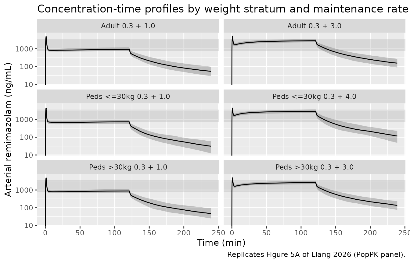
# Replicates Figure 3 of Liang 2026: median profiles at the common
# 0.3 mg/kg + 1.0 mg/kg/h regimen, grouped by the paper's weight bands, showing
# that exposure rises with weight and that the lighter children sit below the
# adult target range.
obs |>
  filter(treatment %in% c("Adult 0.3 + 1.0", "Peds <=30kg 0.3 + 1.0",
                          "Peds >30kg 0.3 + 1.0"),
         time <= 240) |>
  group_by(treatment, time) |>
  summarise(Q50 = quantile(Cc, 0.50), .groups = "drop") |>
  ggplot(aes(time, Q50, colour = treatment)) +
  geom_rect(data = adult_band, inherit.aes = FALSE,
            aes(xmin = -Inf, xmax = Inf, ymin = ymin, ymax = ymax),
            fill = "grey70", alpha = 0.35) +
  geom_line(linewidth = 0.8) +
  scale_y_log10() +
  labs(
    x = "Time (min)", y = "Median arterial remimazolam (ng/mL)",
    colour = NULL,
    title = "Exposure increases with body weight at a fixed mg/kg regimen",
    caption = "Replicates Figure 3 of Liang 2026; grey band is the adult target range (Table 5)."
  ) +
  theme(legend.position = "bottom")
#> Warning in scale_y_log10(): log-10 transformation introduced infinite values.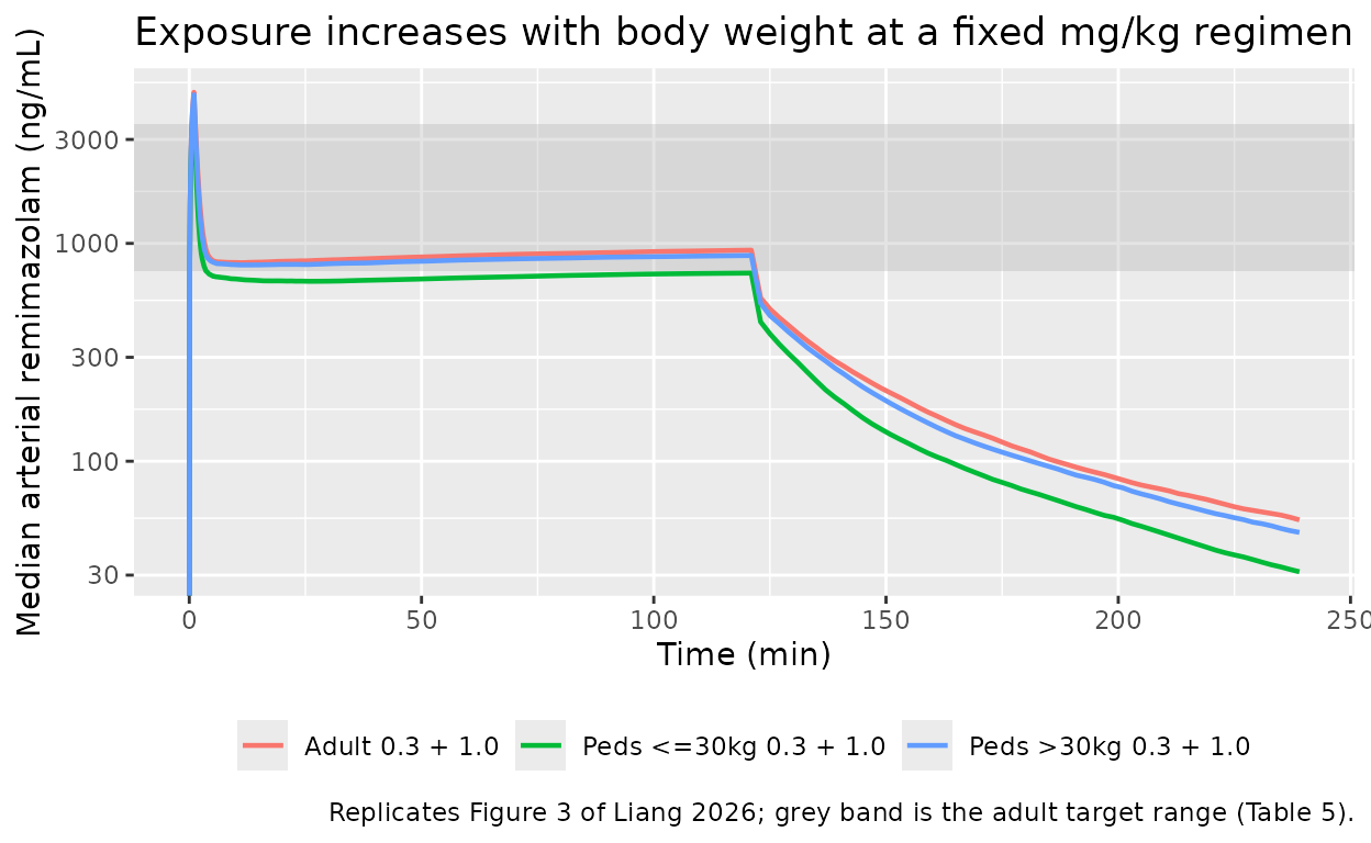
PKNCA validation
Two intervals are needed. ctrough over 0-120 min is the
paper’s C2h (the concentration 2 h after dosing initiation);
cmax, tmax, aucinf.obs and
half.life come from the 0 to infinity interval.
ctrough is NA unless a record sits exactly at
the interval end, which is why tgrid pins t = 120.
# Only `!is.na(Cc)` -- adding `time > 0` or `Cc > 0` would drop the time-zero
# row PKNCA needs to anchor AUC, producing one warning per subject.
sim_nca <- sim |>
  filter(!is.na(Cc)) |>
  select(id, time, Cc, treatment)

# Defensive time-zero guarantee. tgrid already starts at 0 and the infusion
# begins there, so Cc = 0 is the correct pre-dose value; existing rows win.
sim_nca <- bind_rows(
  sim_nca,
  sim_nca |> distinct(id, treatment) |> mutate(time = 0, Cc = 0)
) |>
  distinct(id, treatment, time, .keep_all = TRUE) |>
  arrange(id, treatment, time)

conc_obj <- PKNCA::PKNCAconc(sim_nca, Cc ~ time | treatment + id,
                             concu = "ng/mL", timeu = "min")

# One dose record per infusion; PKNCA needs the total administered amount to
# be consistent with the concentration units.
dose_df <- events |>
  filter(evid == 1) |>
  select(id, time, amt, treatment)

dose_obj <- PKNCA::PKNCAdose(dose_df, amt ~ time | treatment + id,
                             doseu = "mg")

intervals <- data.frame(
  start      = c(0, 0),
  end        = c(120, Inf),
  ctrough    = c(TRUE, FALSE),
  cmax       = c(FALSE, TRUE),
  tmax       = c(FALSE, TRUE),
  aucinf.obs = c(FALSE, TRUE),
  half.life  = c(FALSE, TRUE)
)

nca_res <- PKNCA::pk.nca(PKNCA::PKNCAdata(conc_obj, dose_obj,
                                          intervals = intervals))
# Model time is minutes, so PKNCA returns AUC in ng*min/mL and half-life in
# min. Convert AUC to the ng*h/mL the paper reports before comparing.
nca_tbl <- as.data.frame(nca_res$result) |>
  mutate(PPORRES = if_else(PPTESTCD == "aucinf.obs", PPORRES / 60, PPORRES))
Comparison against published NCA
Adult reference values are Table 5; paediatric values are the PopPK columns of Table 7. The paper reports a single Cmax per weight stratum because Cmax is set by the 0.3 mg/kg induction dose, which is common to both maintenance rates.
published <- tibble::tribble(
  ~treatment,                ~cmax, ~ctrough, ~aucinf.obs,
  "Adult 0.3 + 1.0",          4990,      946,        2320,
  "Adult 0.3 + 3.0",          4990,     2810,        6360,
  "Peds <=30kg 0.3 + 1.0",    4260,      735,        1760,
  "Peds <=30kg 0.3 + 4.0",    4260,     2910,        6340,
  "Peds >30kg 0.3 + 1.0",     4770,      874,        2130,
  "Peds >30kg 0.3 + 3.0",     4770,     2590,        5830
)

cmp <- nlmixr2lib::ncaComparisonTable(
  simulated     = nca_tbl,
  reference     = published,
  by            = "treatment",
  params        = c("cmax", "ctrough", "aucinf.obs"),
  units         = c(cmax = "ng/mL", ctrough = "ng/mL",
                    aucinf.obs = "ng*h/mL"),
  tolerance_pct = 20
)

knitr::kable(
  cmp,
  caption = "Simulated vs. published exposures (Table 5 adults, Table 7 PopPK paediatric). Ctrough is the paper's C2h. * differs from reference by >20%.",
  align   = c("l", "l", "r", "r", "r")
)| NCA parameter | treatment | Reference | Simulated | % diff |
|---|---|---|---|---|
| Cmax (ng/mL) | Adult 0.3 + 1.0 | 4990 | 4940 | -1.0% |
| Cmax (ng/mL) | Adult 0.3 + 3.0 | 4990 | 4960 | -0.6% |
| Cmax (ng/mL) | Peds <=30kg 0.3 + 1.0 | 4260 | 4320 | +1.3% |
| Cmax (ng/mL) | Peds <=30kg 0.3 + 4.0 | 4260 | 4280 | +0.6% |
| Cmax (ng/mL) | Peds >30kg 0.3 + 1.0 | 4770 | 4810 | +0.9% |
| Cmax (ng/mL) | Peds >30kg 0.3 + 3.0 | 4770 | 4800 | +0.7% |
| AUC0-∞ (obs) (ng*h/mL) | Adult 0.3 + 1.0 | 2320 | 2280 | -1.9% |
| AUC0-∞ (obs) (ng*h/mL) | Adult 0.3 + 3.0 | 6360 | 6470 | +1.8% |
| AUC0-∞ (obs) (ng*h/mL) | Peds <=30kg 0.3 + 1.0 | 1760 | 1730 | -1.5% |
| AUC0-∞ (obs) (ng*h/mL) | Peds <=30kg 0.3 + 4.0 | 6340 | 6170 | -2.7% |
| AUC0-∞ (obs) (ng*h/mL) | Peds >30kg 0.3 + 1.0 | 2130 | 2150 | +0.9% |
| AUC0-∞ (obs) (ng*h/mL) | Peds >30kg 0.3 + 3.0 | 5830 | 5890 | +1.1% |
| Ctrough (ng/mL) | Adult 0.3 + 1.0 | 946 | 930 | -1.7% |
| Ctrough (ng/mL) | Adult 0.3 + 3.0 | 2810 | 2860 | +1.6% |
| Ctrough (ng/mL) | Peds <=30kg 0.3 + 1.0 | 735 | 730 | -0.6% |
| Ctrough (ng/mL) | Peds <=30kg 0.3 + 4.0 | 2910 | 2850 | -2.0% |
| Ctrough (ng/mL) | Peds >30kg 0.3 + 1.0 | 874 | 879 | +0.6% |
| Ctrough (ng/mL) | Peds >30kg 0.3 + 3.0 | 2590 | 2620 | +1.1% |
# Tmax and terminal half-life are not reported by the paper; shown for the
# record. Both are in minutes.
nca_tbl |>
  filter(PPTESTCD %in% c("tmax", "half.life")) |>
  group_by(treatment, PPTESTCD) |>
  summarise(median = median(PPORRES, na.rm = TRUE), .groups = "drop") |>
  tidyr::pivot_wider(names_from = PPTESTCD, values_from = median) |>
  rename("Regimen" = treatment,
         "Median Tmax (min)" = tmax,
         "Median terminal t1/2 (min)" = "half.life") |>
knitr::kable(digits = 1, caption = "Simulated Tmax and terminal half-life (not reported in the source).")| Regimen | Median terminal t1/2 (min) | Median Tmax (min) |
|---|---|---|
| Adult 0.3 + 1.0 | 65.1 | 1 |
| Adult 0.3 + 3.0 | 69.6 | 1 |
| Peds <=30kg 0.3 + 1.0 | 50.7 | 1 |
| Peds <=30kg 0.3 + 4.0 | 51.8 | 1 |
| Peds >30kg 0.3 + 1.0 | 62.5 | 1 |
| Peds >30kg 0.3 + 3.0 | 61.6 | 1 |
Gates
# ---- Gate 1: deterministic. AUC0-inf of a typical-value solve must equal
# total dose / CL. Both sides use the SAME parameters, so the only difference
# is trapezoidal error on the NCA side; a tight bound is correct here.
mod_typ <- rxode2::zeroRe(mod)
#> ℹ parameter labels from comments will be replaced by 'label()'
wt_typ  <- 63.4
ev_typ  <- make_arm(1L, wt_typ, 0.3, 1.0, "typical")
sim_typ <- rxode2::rxSolve(mod_typ, events = ev_typ, keep = "WT") |>
  as.data.frame() |>
  filter(!is.na(Cc))
#> ℹ omega/sigma items treated as zero: 'etalcl', 'etalvc', 'etalvp', 'etalq', 'etalvp2', 'etalq2'
# rxSolve omits `id` entirely for a single-subject event table; PKNCA's
# grouping formula needs it.
if (is.null(sim_typ$id)) sim_typ$id <- 1L

cl_typ    <- 1.03 * (wt_typ / 62)^0.75          # L/min, Table 4 + Equation 3
dose_typ  <- 0.3 * wt_typ + 1.0 * wt_typ * 2    # mg, induction + 2 h maintenance
auc_exact <- dose_typ * 1000 / cl_typ / 60      # ng*h/mL

auc_nca <- PKNCA::pk.nca(PKNCA::PKNCAdata(
  PKNCA::PKNCAconc(sim_typ |> select(id, time, Cc), Cc ~ time | id),
  PKNCA::PKNCAdose(data.frame(id = 1L, time = 0, amt = dose_typ),
                   amt ~ time | id),
  intervals = data.frame(start = 0, end = Inf, aucinf.obs = TRUE)
))
auc_nca_h <- as.data.frame(auc_nca$result) |>
  filter(PPTESTCD == "aucinf.obs") |>
  pull(PPORRES) / 60

auc_err_pct <- 100 * (auc_nca_h - auc_exact) / auc_exact
cat(sprintf("closed-form AUC0-inf %.1f vs NCA %.1f ng*h/mL (%.3f%%)\n",
            auc_exact, auc_nca_h, auc_err_pct))
#> closed-form AUC0-inf 2320.4 vs NCA 2322.2 ng*h/mL (0.078%)
# Pure numerical (trapezoidal) error against the model's own closed form.
stopifnot(abs(auc_err_pct) < 1)

# The same closed form against the paper's printed Table 5 value of 2320
# ng*h/mL. This one number pins the reference weight (62 vs 63 kg), the CL
# estimate, the 0.75 exponent, the 1000x ng/mL scaling and the dose
# interpretation simultaneously.
stopifnot(abs(100 * (auc_exact - 2320) / 2320) < 1)

# ---- Gate 2: cohort medians against the paper. Assert the CENTRE and an
# envelope, never the extremes of a random cohort. Realised across the 18
# comparisons: median |% diff| 1.1 and max 2.7 on one draw, max 2.9 on
# another. Bounds of 10 and 15 leave room for a different cohort draw while
# still going red on a mis-transcribed dose, volume or unit, which move these
# by tens of percent. Do not tighten these to one observed run.
pct <- as.numeric(sub("%", "", cmp$`% diff`))
pct <- pct[!is.na(pct)]
stopifnot(length(pct) == 18L)
cat(sprintf("median |%% diff| %.2f ; max |%% diff| %.2f (n = %d)\n",
            median(abs(pct)), max(abs(pct)), length(pct)))
#> median |% diff| 1.10 ; max |% diff| 2.70 (n = 18)
stopifnot(median(abs(pct)) < 10)
stopifnot(max(abs(pct)) < 15)

# ---- Gate 3: mass balance. Essentially all drug has left the system by the
# end of the grid, so aucinf.obs is not extrapolating a meaningful fraction.
last_row <- sim_typ[which.max(sim_typ$time), ]
frac_left <- with(last_row, central + peripheral1 + peripheral2) / dose_typ
cat(sprintf("fraction of dose remaining at t = %.0f min: %.3g\n",
            last_row$time, frac_left))
#> fraction of dose remaining at t = 720 min: 0.000285
stopifnot(frac_left < 0.001)
Assumptions and deviations
Three items resolve against the supplementary NONMEM control stream rather than the main text. The supplement (Section S2) contains the final control stream, which settles each of them; all three were verified against it.
-
The residual error is additive on the LOG scale, not on the
concentration scale. Equation 5 prints
Cij = CTV,ij + eps_aijwithsigma^2 = 0.0162, which taken literally is an additive SD of 0.127 ng/mL against concentrations reaching 5790 ng/mL – implausible, and contradicted by goodness-of-fit plots drawn on log axes (Figure S3). The control stream resolves it: its$PROBLEMdescription readslogDV+ADD,$ERRORsetsIPRED = LOG(F)and returnsY = IPRED * (1 + ERR(1)) + ERR(2), and$SIGMAfixes the proportional term to0 FIX, leaving only the additive term on the log scale. That is nlmixr2’sCc ~ lnorm(expSd)withexpSd = sqrt(0.0162) = 0.127, i.e. roughly 12.8% CV – a sensible assay plus model-misspecification magnitude. The inert0 FIXproportional term is not encoded: it multiplieslog(F)rather thanF, so it has noprop()equivalent, and being fixed at zero it contributes nothing. -
The allometric reference weight is 62 kg, not the 63 kg of
Table 4’s row headers. The control stream centres every term on
(WEIGHTBL/62)and labels its own thetasL/min/62 kg; the analysis-population median was 62.8 kg (Table S1). 62 kg is used here. The choice is not cosmetic but it is small – a 1.3% scale factor on volumes and 1.0% on clearances – and Gate 1 above confirms 62 kg is the value that reproduces Table 5’s printed AUC0-inf of 2320 ng*h/mL to better than 1%. -
Q2 carries inter-individual variability, despite Equation
4’s prose list. Equation 4 names CL, V1, V2, V3 and Q3 as the
parameters with IIV, omitting Q2. Table 4 nonetheless reports
omega^2 (Q2) = 0.107with good precision (RSE 18.3%, shrinkage 5%) and aomega (V2):omega (Q2)covariance, and the control stream declaresETA(4)on Q2 inside an$OMEGA BLOCK(2). The prose list is simply incomplete; all six disposition parameters carry IIV here.
Further items.
- The induction and maintenance infusions are sequential, not concurrent. The paper describes “an induction bolus of 0.3 mg/kg administered over 1 min, followed by continuous maintenance infusions”, without stating whether the maintenance starts at t = 0 or at t = 1 min. Tables 5 and 7 settle it: each reports a single Cmax shared by both maintenance rates. That can only hold if no maintenance drug has been delivered by the time of the peak, so the maintenance infusion is encoded here as starting when the induction infusion ends. Simulating them concurrently instead raises the 3.0 mg/kg/h arm’s Cmax about 15% above the 1.0 mg/kg/h arm’s and breaks the agreement with Table 5.
-
The companion PBPK model is not packaged. The
paper’s PBPK half was built in PK-Sim v12 and publishes only a six-row
drug-specific parameter table (Table 2: molecular weight, logP, pKa,
fraction unbound, an optimised organ-specific permeability of 4.01e-4
cm/min, and a CES1 specific clearance of 50.37 1/min). No ODE system,
compartment list, organ volume, blood flow or tissue-plasma partition
coefficient is reported – the partition-coefficient and
cellular-permeability rows read “diverse / PK-Sim standard”, naming
methods rather than values – and no PK-Sim project file is deposited
with the supplement. Reconstructing it would require substituting the
platform’s built-in physiology and CES1 tissue-expression libraries from
outside any available source, which this repository does not do. The
PBPK-specific content that is published is preserved instead:
Table 2’s parameters and the CES1 ontogeny function are recorded in the
model file’s
descriptionand in theFCES1entry ofcovariatesDataExcluded. -
CES1 ontogeny is absent from this model by the authors’ own
design. The maturation function of Equation 2
(
Fbirth0.20,Adultmax1,Age501.10 years,n0.56) was tested on CL and rejected: the analysis population was entirely adult and CES1-mature, so FCES1 spanned only 0.862-0.916 across subjects (Table S1) and changed the OFV negligibly. The consequence for reuse is a real limitation the paper acknowledges – below about 3 years of age, where CES1 is genuinely immature, this PopPK model scales clearance by weight alone and will overpredict clearance (and so underpredict exposure). The paper’s own trial enrols from 3 years upward for this reason. -
No covariate other than weight is in the model. Sex
on V2, BUN on CL and albumin on V1 all entered the full model during
forward inclusion and all three were dropped in backward elimination
(Table S3). They are documented in
covariatesDataExcludedwith their dOFV values so the screen’s provenance survives; none is referenced inmodel(). - Paediatric weight distributions are approximated as uniform. Table S5 reports only median [min, max] per stratum. A uniform draw over the reported range has expected medians of about 20.6 and 50.0 kg against the paper’s 20.3 and 46.3 kg, so the heavier stratum in particular is simulated a few kilograms above the paper’s cohort. That accounts for most of the small positive bias in the “Peds >30kg” rows of the comparison table.
-
Race is recorded as 100% Asian. Both studies
enrolled Chinese subjects only (Table 1). The model carries no race
term, so this affects only the
populationmetadata. -
Reported minor inconsistencies in the source, none affecting
the model.
- Results 3.1 states 14 females (19.7%) and 57 males (80.3%), while
Table S1 reports 15 female (21.1%) and 56 male (78.9%); Table S1 is
internally consistent with its own per-study counts (12 of 63 plus 3 of
8), so its values are used. (b) Table 4’s “Final Model 95% CI” cell for
omega^2 (Q3)reads 0.0139-0.0267, which is a duplicate of theomega^2 (CL)row’s interval and cannot bracket the 0.0777 point estimate; the bootstrap column’s 0.0442-0.122 is consistent. Only the point estimate is used here, so the erroneous interval has no effect. (c) The tabulated eGFR values (median 48.3 mL/min in healthy young adults, Table S1) are not reproducible from the MDRD form printed as Equation 6, which evaluates to about 124 mL/min for the median subject. eGFR was rejected as a covariate, so this affects nothing in the model; it is flagged in theCRCLentry ofcovariatesDataExcludedin case that column is ever reused.
- Results 3.1 states 14 females (19.7%) and 57 males (80.3%), while
Table S1 reports 15 female (21.1%) and 56 male (78.9%); Table S1 is
internally consistent with its own per-study counts (12 of 63 plus 3 of
8), so its values are used. (b) Table 4’s “Final Model 95% CI” cell for
- The model predicts arterial concentrations. See Population. A venous prediction is not available from this model.
- Flumazenil co-administration is not modelled. HR7056-Ib subjects received 0.5 mg flumazenil or saline 1 h 55 min into dosing. Flumazenil is a receptor antagonist with no reported effect on remimazolam disposition, and the source model carries no term for it.