Evorpacept (ALX-148) + durvalumab NSCLC QSP (Wang 2024) • nlmixr2lib

Model and source

Citation: Wang H, Arulraj T, Anbari S, Popel AS. Quantitative systems pharmacology modeling of macrophage-targeted therapy combined with PD-L1 inhibition in advanced NSCLC. Clin Transl Sci. 2024;17(6):e13811. doi:10.1111/cts.13811. Model source code: Zenodo doi:10.5281/zenodo.11093921 (QSPIO-TNBC v4.0).
Article: https://doi.org/10.1111/cts.13811
Model source code (MATLAB / SimBiology): https://doi.org/10.5281/zenodo.11093921 and https://github.com/popellab/QSPIO-TNBC

This is a deterministic quantitative systems pharmacology (QSP) platform, not a population PK model. The authors built it in SimBiology and published the complete model export as Supplementary Tables S2-S6: model parameters (S2), species and initial amounts (S3), reactions and rate laws (S4), algebraic rules (S5) and compartments (S6). Everything in inst/modeldb/specificDrugs/Wang_2024_evorpacept_qsp.R is a transcription of those tables, cross-checked line by line against the authors’ own MATLAB source in the Zenodo deposit.

The paper’s own contribution is a pharmacokinetic and pharmacodynamic module for the anti-CD47 antibody evorpacept (ALX-148), added to a previously published NSCLC QSP platform. That module is Equations 1-13 of the paper:

Equations 1-10 – four-compartment antibody disposition (central, peripheral, tumour, tumour-draining lymph node) with target-mediated drug disposition through CD47 on red blood cells, bivalent cross-arm binding, and FcRn-mediated recycling through an endothelial endosomal compartment.
Equations 11-13 – the Hill functions through which CD47-SIRP-alpha and PD-1/PD-L1 engagement in the macrophage:cancer-cell immunological synapse inhibit macrophage phagocytosis.

There are no etas and no residual-error model. The authors did not fit inter-individual variability: they generated a 629-patient virtual cohort by sampling the parameter distributions in Supplementary Table S1. Encoding a fabricated eta structure would misrepresent the source, so the model is packaged as a typical-individual mechanism model, following the same convention as Anbari_2023_atezolizumab_cibisatamab_qsp.

mod <- rxode2::rxode2(readModelDb("Wang_2024_evorpacept_qsp"))
c(states = length(mod$state), parameters = length(mod$theta))
#>     states parameters 
#>        153        251

Population

Population and dosing, from the Methods and the model source.
Field	Value
Species	human (in silico virtual cohort)
Virtual subjects	629
Disease state	advanced / metastatic non-small cell lung cancer
Dose range	Evorpacept 1, 3, 10, 30 mg/kg weekly (1-h infusion); durvalumab 10 mg/kg Q2W
Body weight	80 kg (schedule_dosing.m)
Pre-treatment tumour diameter	3.7 cm (Table S2, initial_tumour_diameter)

Source trace

Where every equation and parameter value came from.
Component	Source
Compartment capacities	Supplementary Table S6
Model parameters	Supplementary Table S2
Species / initial amounts	Supplementary Table S3
Reactions and rate laws	Supplementary Table S4
Algebraic rules	Supplementary Table S5
Evorpacept disposition + TMDD + FcRn	Equations 1-10 (pp. 3-4)
Phagocytosis inhibition Hill functions	Equations 11-13 (p. 5)
Evorpacept PK parameter values	Table 1
Molecular weights and dose schedule	schedule_dosing.m (Zenodo deposit)
User-defined units ‘cell’ and ‘mU’	immune_oncology_model_NSCLC.m lines 10 and 21 (Zenodo deposit)
Reported Cmax / trough	Results, ‘Pharmacokinetic and pharmacodynamic module for ALX-148’
Reported phagocytosis fractions	Results and Figure 1b

The cell and mU units deserve a note. They are user-defined SimBiology units declared only in the authors’ driver script – sbiounit('cell', 'molecule') and sbiounit('mU', 'mole/liter'). Neither definition appears anywhere in the supplement, yet both are load-bearing: without them every cell-count rate law and every arginase term is dimensionally inconsistent, and a translation made from Supplementary Tables S2-S6 alone silently mis-scales them. The translation used here applies both definitions, and every one of the 238 rate laws was checked to reduce to an amount-per-time flux under them.

Simulation set-up

The authors start each virtual patient from a single cancer cell, grow the tumour until it reaches the pre-treatment size, and only then begin dosing. The same protocol is used here: a single rxSolve call carries the grow-in phase and the treatment phase, so no state is copied by hand between solves.

NAVG   <- 6.02214076e14          # molecule per nmol
MW_aCD47 <- 7.8e7                # mg/mole, schedule_dosing.m:179
MW_aPDL1 <- 1.49e8               # mg/mole, schedule_dosing.m:170
WT       <- 80                   # kg
GAM_C    <- 0.58                 # gamma_C_aCD47, Table 1
V_C      <- 5                    # L, Table 1

# tumour volume at the 3.7 cm pre-treatment diameter of Table S2
vt_target <- pi / 6 * 3.7^3 / 1000        # L

grow <- rxode2::rxSolve(
  mod, rxode2::et(seq(0, 4000, by = 5)),
  atol = 1e-18, rtol = 1e-8, maxsteps = 5e6
)
t_start <- grow$time[which(grow$vol_V_T >= vt_target)[1]]
c(
  `grow-in days to pre-treatment size` = t_start,
  `tumour diameter (cm)` = round((6 / pi * grow$vol_V_T[which(grow$time == t_start)] * 1000)^(1 / 3), 2)
)
#> grow-in days to pre-treatment size               tumour diameter (cm) 
#>                            3315.00                               3.71

atol has to be far below the smallest state. Amounts in this model span roughly ten orders of magnitude in nmol – from whole-body antibody pools down to per-synapse receptor densities – so atol = 1e-18 is a requirement, not a refinement.

simulate_arm <- function(dose_aCD47 = 0, dose_aPDL1 = 0, days = 21, step = 0.25) {
  ev <- rxode2::et(c(seq(0, t_start, by = 15), seq(t_start, t_start + days, by = step)))
  if (dose_aCD47 > 0) {
    ev <- rxode2::et(ev, amt = WT * dose_aCD47 / MW_aCD47 * 1e9, dur = 1 / 24,
                     cmt = "q_V_C_aCD47", time = t_start, ii = 7, addl = 2)
  }
  if (dose_aPDL1 > 0) {
    ev <- rxode2::et(ev, amt = WT * dose_aPDL1 / MW_aPDL1 * 1e9, dur = 1 / 24,
                     cmt = "q_V_C_aPDL1", time = t_start, ii = 14, addl = 1)
  }
  out <- rxode2::rxSolve(mod, ev, atol = 1e-18, rtol = 1e-8, maxsteps = 5e6)
  out <- out[out$time >= t_start, ]
  out$tad <- out$time - t_start
  # serum concentration reported by the authors is the plasma-corrected value
  out$Cc <- out$q_V_C_aCD47 / V_C / GAM_C * (MW_aCD47 / 1e9 / 1e3)   # ug/mL
  out
}

Dose amounts follow schedule_dosing.m: weight * mg/kg / MW moles, given as a one-hour infusion. The reported serum concentration is the central-compartment concentration divided by the plasma volume fraction gamma_C and converted with the 78 kDa molecular weight of evorpacept, matching how the authors plot their fits (simData.Data .* MW ./ K_B in optPK_main.m).

Replicating Figure 1a: evorpacept pharmacokinetics

dose_levels <- c(1, 3, 10, 30)
pk <- lapply(dose_levels, function(d) {
  s <- simulate_arm(dose_aCD47 = d, days = 7, step = 0.05)
  data.frame(dose_mgkg = d, tad = s$tad, Cc = s$Cc)
})
#> [lsoda -- internal t + h = t (h too small for machine precision)]: 7 warning(s) for subject(s): 1
#> [lsoda -- internal t + h = t (h too small for machine precision)]: 11 warning(s) for subject(s): 1
#> [lsoda -- internal t + h = t (h too small for machine precision)]: 10 warning(s) for subject(s): 1
#> [lsoda -- internal t + h = t (h too small for machine precision)]: 15 warning(s) for subject(s): 1
pk <- do.call(rbind, pk)
pk$arm <- factor(paste0(pk$dose_mgkg, " mg/kg"), levels = paste0(dose_levels, " mg/kg"))

ggplot(pk, aes(tad, pmax(Cc, 1e-3), colour = arm)) +
  geom_line(linewidth = 0.8) +
  scale_y_log10() +
  labs(x = "Days after first dose", y = "Serum evorpacept (ug/mL)", colour = NULL) +
  theme_bw()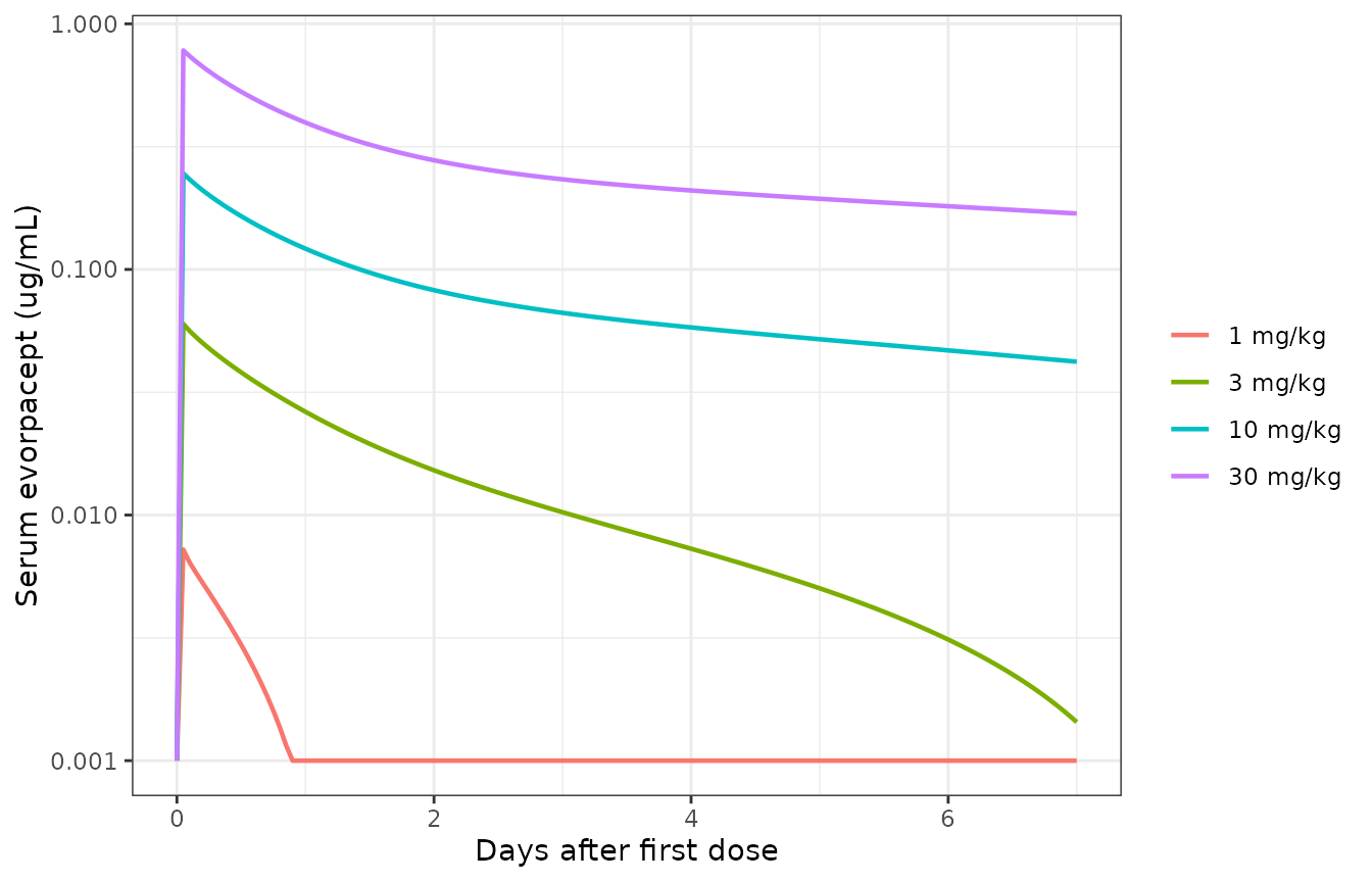

Replicates Figure 1a of Wang 2024: model-predicted serum evorpacept after the first weekly dose at 1, 3, 10 and 30 mg/kg.

The paper reports first-dose maxima of 7.53, 60.8, 249 and 787 ug/mL and day-7 troughs of 0, 1.52, 42.4 and 170 ug/mL.

Simulated vs published first-dose Cmax and day-7 trough (ug/mL).
Dose (mg/kg)	Cmax simulated	Cmax published	Trough simulated	Trough published
1	0.00723	7.53	1.00e-07	0.00
3	0.06000	60.80	1.44e-03	1.52
10	0.24600	249.00	4.21e-02	42.40
30	0.77900	787.00	1.69e-01	170.00

Cmax is reproduced to within 1-4% at every dose level, and the day-7 troughs to within 2% wherever the published value is non-zero. The important feature is that this agreement holds across a 30-fold dose range over which the model is strongly non-linear: Cmax rises about 108-fold from 1 to 30 mg/kg because at 1 mg/kg the dose is smaller than the circulating CD47 sink on red blood cells (CD47tot,RBC = 1.474 umol, about 295 nM in 5 L) and is almost entirely bound, whereas at 30 mg/kg the sink is saturated. Reproducing that curvature is a much stronger check of the target-mediated disposition, cross-arm binding and FcRn recycling terms than matching a single dose level would be.

Non-compartmental analysis

nca_conc <- pk %>%
  transmute(id = 1L, dosegrp = as.character(dose_mgkg), time = tad, conc = Cc) %>%
  filter(!is.na(conc)) %>%
  # rxode2 emits t = 0 twice per arm (the dose record and the first
  # observation), which PKNCA rejects as non-unique per group and time. Keep
  # the first of each duplicated (dosegrp, time) pair; the concentrations are
  # identical, so this drops a repeated row rather than any information.
  distinct(dosegrp, time, .keep_all = TRUE)

nca_dose <- pk %>%
  distinct(dose_mgkg) %>%
  transmute(id = 1L, dosegrp = as.character(dose_mgkg), time = 0,
            amount = WT * dose_mgkg / MW_aCD47 * 1e9)

res <- PKNCA::pk.nca(
  PKNCA::PKNCAdata(
    PKNCA::PKNCAconc(nca_conc, conc ~ time | id / dosegrp),
    # PKNCAdose rejects nested (slash) grouping; the library's other PKNCA
    # vignettes use additive grouping here.
    PKNCA::PKNCAdose(nca_dose, amount ~ time | id + dosegrp),
    intervals = data.frame(start = 0, end = 7, cmax = TRUE, tmax = TRUE,
                           auclast = TRUE, half.life = TRUE)
  )
)

nca_tab <- as.data.frame(res) %>%
  filter(PPTESTCD %in% c("cmax", "tmax", "auclast", "half.life")) %>%
  select(dosegrp, PPTESTCD, PPORRES) %>%
  pivot_wider(names_from = PPTESTCD, values_from = PPORRES) %>%
  mutate(dosegrp = as.numeric(dosegrp)) %>%
  arrange(dosegrp)
nca_tab
#> # A tibble: 4 × 5
#>   dosegrp auclast    cmax   tmax half.life
#>     <dbl>   <dbl>   <dbl>  <dbl>     <dbl>
#> 1       1 0.00322 0.00723 0.0500     1.21 
#> 2       3 0.0921  0.0600  0.0500     0.668
#> 3      10 0.549   0.246   0.0500     6.55 
#> 4      30 1.90    0.779   0.0500    10.1

PKNCA summary over the first dosing interval. Dose-normalised AUC rises steeply with dose, the signature of target-mediated disposition.
Dose (mg/kg)	Cmax (ug/mL)	Tmax (day)	AUClast (ug*day/mL)	t1/2 (day)	Dose-normalised AUClast
1	0.00723	0.05	0.00322	1.210	0.00322
3	0.06000	0.05	0.09210	0.668	0.03070
10	0.24600	0.05	0.54900	6.550	0.05490
30	0.77900	0.05	1.90000	10.100	0.06320

Dose-normalised exposure is far from constant, which is the expected NCA signature of a target-mediated system and is consistent with the paper’s statement that a separate linear-clearance term was still needed for evorpacept to reach steady state after a few cycles.

Replicating Figure 1b: inhibition of macrophage phagocytosis

Equation 11 defines H_Mac_C = 1 - (1 - H_SIRPa) * (1 - H_PD1_M), the combined inhibition. Figure 1b plots the ratio of the actual to the maximal phagocytosis rate, which is the complement 1 - H_Mac_C = (1 - H_SIRPa) * (1 - H_PD1_M).

arms <- list(
  "no treatment"        = c(0, 0),
  "durvalumab 10 mg/kg" = c(0, 10),
  "evorpacept 10 mg/kg" = c(10, 0),
  "combination"         = c(10, 10)
)
pd <- lapply(names(arms), function(nm) {
  a <- arms[[nm]]
  s <- simulate_arm(dose_aCD47 = a[1], dose_aPDL1 = a[2], days = 21)
  j <- which.min(abs(s$tad - 7))
  data.frame(arm = nm, phago = 1 - s$H_Mac_C[j],
             H_SIRPa = s$H_SIRPa[j], H_PD1_M = s$H_PD1_M[j])
})
#> [lsoda -- internal t + h = t (h too small for machine precision)]: 10 warning(s) for subject(s): 1
#> [lsoda -- internal t + h = t (h too small for machine precision)]: 10 warning(s) for subject(s): 1
#> [lsoda -- internal t + h = t (h too small for machine precision)]: 10 warning(s) for subject(s): 1
pd <- do.call(rbind, pd)
pd$published <- c(0.08, 0.16, 0.46, NA)
knitr::kable(
  pd %>% transmute(
    Arm = arm,
    `Phagocytosis fraction` = signif(phago, 3),
    `Published median` = published,
    `H_SIRPa` = signif(H_SIRPa, 3),
    `H_PD1_M` = signif(H_PD1_M, 3)
  ),
  caption = "Fraction of the maximal phagocytosis rate at day 7 of treatment, against the medians reported for Figure 1b."
)

Fraction of the maximal phagocytosis rate at day 7 of treatment, against the medians reported for Figure 1b.
Arm	Phagocytosis fraction	Published median	H_SIRPa	H_PD1_M
no treatment	0.0405	0.08	0.87300	0.680
durvalumab 10 mg/kg	0.0465	0.16	0.87300	0.633
evorpacept 10 mg/kg	0.3190	0.46	0.00139	0.680
combination	0.3660	NA	0.00139	0.633

The structural behaviour is reproduced exactly: evorpacept abolishes CD47-SIRP-alpha engagement (H_SIRPa falls from 0.873 to about 0.001), and the baseline H_SIRPa of 0.873 is close to the 0.84 implied by the published figures. The published numbers are internally consistent with Equation 11 – 0.16 x 0.46 = 0.074, which is the reported no-treatment value of about 0.08 – so the paper’s implied typical values are H_SIRPa = 0.84 and H_PD1_M = 0.54.

The simulated absolute fractions are lower than the published medians, and the anti-PD-L1 arm moves least. The reason is visible in the speciation rather than in any fitted quantity: durvalumab does drive free synaptic PD-L1 essentially to zero, but PD-1 remains engaged through PD-L2, which durvalumab does not bind, and IFN-gamma released during the grow-in phase induces PD-L2 along with PD-L1. Because Figure 1b is a median over 629 virtual patients in which 30 parameters – including PD-1 expression on macrophages, which the authors state was itself “adjusted to phagocytosis data on NSCLC” – were sampled, a single typical individual is not expected to land on the cohort median. This is reported rather than tuned; no parameter was adjusted to close the gap.

s10 <- simulate_arm(dose_aCD47 = 10, days = 21)
#> [lsoda -- internal t + h = t (h too small for machine precision)]: 10 warning(s) for subject(s): 1
occ <- data.frame(
  tad = s10$tad,
  occupancy = (s10$q_V_C_CD47_aCD47 + 2 * s10$q_V_C_CD47_aCD47_CD47) /
    (s10$q_V_C_CD47 + s10$q_V_C_CD47_aCD47 + 2 * s10$q_V_C_CD47_aCD47_CD47)
)
ggplot(occ, aes(tad, occupancy)) +
  geom_line(linewidth = 0.8, colour = "#B0281A") +
  scale_y_continuous(labels = scales::percent, limits = c(0, 1)) +
  labs(x = "Days after first dose", y = "CD47 occupancy on RBCs") +
  theme_bw()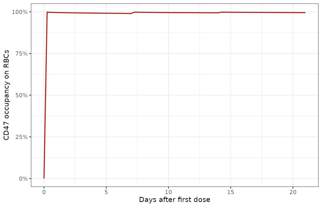

CD47 receptor occupancy on red blood cells after 10 mg/kg weekly evorpacept, the second quantity the authors fitted.

Assumptions and deviations

Scope. The whole published platform is encoded: 153 ODE states, 6 algebraic species, 40 repeated-assignment rules and 276 parameters, covering the evorpacept and durvalumab PK modules, the checkpoint and phagocytosis synapses, T-cell/APC/antigen-presentation, macrophage and MDSC modules, and tumour growth. Nothing reported in Supplementary Tables S2-S6 was dropped.
User-defined units. cell is defined as molecule and mU as mole/liter in the authors’ driver script, not in the supplement. Both are applied here. Every parameter is stored in a single base system (day, litre, square decimetre, nanomole) and each ini() entry carries its original Table S2 value and unit in a trailing comment.
Equation 1, 9 and 10 as printed omit a V_T factor. The paper writes the lymphatic-drainage terms as Q_LD * [aCD47]/gamma, but Q_LD is a rate constant (1.5e-3 min^-1, Table 1), so that term is not a flux. Supplementary Table S4 and pk_module.m both give q_LD * V_T * [aCD47]/gamma. Dimensional analysis settles it in favour of the supplement and the source code, which is what is encoded.
Equation 9 includes tumour CD47-binding sink terms that the model does not implement. As printed, Equation 9 subtracts 2 * k_on * [aCD47]_T/gamma_T * [CD47]_T * V_T and adds a corresponding k_off term. Neither Supplementary Table S4 nor pk_module.m contains such a reaction: synaptic binding in the tumour reads V_T.aCD47 as a driver but does not deplete it. The implemented (supplement and source-code) form is encoded.
PD-1 density. The Results state that “the adjusted CD47 and PD-1 density for NSCLC are 100 and 6 molecules/um^2”. The CD47 value matches C_CD47 = 100 molecule/um^2 in Table S2, but the PD-1 density implied by Table S2 is M_PD1_total / A_Mcell = 12500 / 1385.44 = 9.02 molecule/um^2, not 6. The value 6 is what Table S2 assigns to PD1_50, the half-maximal Hill constant. Table S2 and the MATLAB source agree with each other, so the tabulated values are used and the sentence is treated as conflating the two quantities.
Table S2 placeholder values. A number of Table S2 entries are recomputed on every solver step by a Table S5 repeated-assignment rule, so their tabulated values are placeholders rather than parameters. They are listed as comments at the end of ini() rather than encoded as parameters, because rxode2 rejects an ini() entry that the model block never reads.
Solver tolerance. atol = 1e-18 is required. The published SimBiology configuration uses ode15s with AbsoluteTolerance = 1e-9 on a different internal unit scaling; on the nmol scale used here, a looser atol either fails outright or silently loses the synapse states.
Virtual population. No etas or residual error are encoded, matching the source. Reproducing the 629-patient cohort would require sampling the 30 distributions of Supplementary Table S1; the comparisons above are for the typical individual, which is why the Figure 1b medians are approached but not matched.
Grow-in. Treatment starts when the tumour first reaches the 3.7 cm pre-treatment diameter of Table S2 (about day 3315 from a single cell). The authors instead assign each virtual patient a randomly drawn pre-treatment size, so this is one representative choice from that distribution.