Piperaquine (Tarning 2014)
Source:vignettes/articles/Tarning_2014_piperaquine.Rmd
Tarning_2014_piperaquine.RmdModel and source
- Citation: Tarning J, Lindegardh N, Lwin KM, Annerberg A, Kiricharoen L, Ashley E, White NJ, Nosten F, Day NPJ (2014). Population Pharmacokinetic Assessment of the Effect of Food on Piperaquine Bioavailability in Patients with Uncomplicated Malaria. Antimicrobial Agents and Chemotherapy 58(4):2052-2058. doi:10.1128/AAC.02318-13.
- Article: https://doi.org/10.1128/AAC.02318-13
The package model can be loaded with:
mod_fn <- readModelDb("Tarning_2014_piperaquine")
mod    <- rxode2::rxode2(mod_fn())
Population
The Tarning 2014 study enrolled 30 adults aged 16-65 years with uncomplicated Plasmodium falciparum malaria at the Shoklo Malaria Research Unit in Mae Sot, Thailand, randomised 15:15 to a fasting arm and a fed arm. All patients received the standard fixed-dose oral dihydroartemisinin-piperaquine combination (DuoCotecxin: 40 mg dihydroartemisinin + 320 mg piperaquine phosphate per tablet) once daily for three days, titrated to a daily target dose of 18 mg piperaquine phosphate/kg. Patients in the fed arm consumed a 200 mL carton of chocolate milk containing 6.4 g of fat with each dose; patients in the fasting arm received study medication after at least 2 hours of fasting and were asked to continue fasting for 3 hours post-dose. Demographics from Table 1 (median [range]): body weight 50 [39-62] kg (fasting) and 53 [45-73] kg (fed); age 38 [18-55] years (fasting) and 28 [19-45] years (fed); 13 male and 2 female in each arm (26.7% female overall). Sampling was dense post-dose: pre-dose and at 0.5, 1, 2, 3, 4, 7, and 24 h after dose 1; 1, 3, 4, 5, 7, and 24 h after dose 2; 1, 2, 3, 4, 5, 6, 8, and 12 h after dose 3; plus follow-up venous samples on days 4, 5, 7, 14, 21, 28, 42, 56, 70, 84, 98, 112, and 126. The final analysis used 985 post-dose piperaquine plasma concentrations after omitting 91 (9.1%) below-the-limit-of-quantification samples (1.2 ng/mL LLOQ), the majority (82.6%) in the long terminal phase beyond day 70.
The same information is available programmatically via the model’s
population metadata
(readModelDb("Tarning_2014_piperaquine")()$population after
the model is loaded).
Source trace
Every parameter and equation traces back to the Tarning 2014
publication; the full citation is in the model file’s
reference field. Per-parameter source locations are
recorded inline in
inst/modeldb/specificDrugs/Tarning_2014_piperaquine.R next
to each ini() entry. The table below collects them in one
place for review.
| Equation / parameter | Value | Source location |
|---|---|---|
lcl = log(67.6) (CL/F, L/h at WT = 70 kg) |
67.6 | Table 2 ‘Value’ (RSE 11.6%; 95% CI 54.0-85.5) |
lvc = log(3030) (Vc/F, L at WT = 70 kg) |
3030 | Table 2 (RSE 16.4%; 95% CI 2160-4180) |
lq = log(408) (Q1/F, L/h at WT = 70 kg) |
408 | Table 2 (RSE 15.0%; 95% CI 309-557) |
lvp = log(6240) (Vp1/F, L at WT = 70 kg, AGE = 33
y) |
6240 | Table 2 (RSE 14.6%; 95% CI 4890-8530) |
lq2 = log(109) (Q2/F, L/h at WT = 70 kg) |
109 | Table 2 (RSE 13.6%; 95% CI 83.3-143) |
lvp2 = log(24400) (Vp2/F, L at WT = 70 kg) |
24400 | Table 2 (RSE 10.1%; 95% CI 20000-29500) |
lmtt = log(2.04) (MTT, h) |
2.04 | Table 2 (RSE 7.50%; 95% CI 1.80-2.41) |
lfdepot = fixed(log(1)) (F) |
1 (fixed) | Table 2 ‘F (%) = 100 (fixed)’ |
e_wt_cl = fixed(0.75) (allometric on CL/Q) |
0.75 (fixed) | Methods page 2053: ‘allometric function with power values of 3/4 for clearance parameters’ |
e_wt_vc = fixed(1.00) (allometric on V) |
1.00 (fixed) | Methods page 2053: ‘and 1 for volume parameters’ |
e_age_vp = 0.0410 (Age effect on Vp1, /year) |
4.10%/y | Table 2 ‘Age effect on Vp1 (%)’ = 4.10 (RSE 18.1%; 95% CI 2.38-5.32) |
e_doseocc_f = 0.253 (Dose-occasion effect on F) |
25.3%/dose | Table 2 ‘Dose effect on F (%)’ = 25.3 (RSE 34.4%; 95% CI 9.82-53.2) |
etalcl ~ 0.057846 (var, log-scale) |
CV 24.4% (IIV) | Table 2 IIV CL (RSE 26.0%); variance = log(0.244^2 + 1) |
etalvc ~ 0.234710 (var, log-scale) |
CV 51.6% (IIV) | Table 2 IIV Vc (RSE 32.3%); variance = log(0.516^2 + 1) |
etalvp ~ 0.188103 (var, log-scale) |
CV 45.6% (IIV) | Table 2 IIV Vp1 (RSE 48.8%); variance = log(0.456^2 + 1) |
etalq2 ~ 0.064375 (var, log-scale) |
CV 25.8% (IIV) | Table 2 IIV Q2 (RSE 48.2%); variance = log(0.258^2 + 1) |
etalmtt ~ 0.056498 (var, log-scale) |
CV 24.1% (BSV; 39.4% IOV not encoded) | Table 2 IIV MTT (RSE 52.7%); variance = log(0.241^2 + 1) |
etalfdepot ~ 0.212074 (var, log-scale) |
CV 48.8% (IOV as forward-sim IIV) | Table 2 IIV F (RSE 16.6%); variance = log(0.488^2 + 1) |
propSd = 0.307 (SD, log-scale) |
sigma 30.7% | Table 2 ‘sigma (% CV)’ = 30.7 (RSE 4.42%; 95% CI 27.8-33.5) |
3 transit compartments fixed; ktr = 4 / MTT
|
– | Methods + Results page 2054: ‘A transit compartment (n = 3) absorption model’ and ‘absorption rate from the last transit compartment could be set as identical to the rate constant between transit compartments’; Savic 2007 convention |
Three-compartment disposition (central,
peripheral1, peripheral2) |
– | Results page 2054: ‘Piperaquine population pharmacokinetics were well described by a 3-compartment distribution model’; Figure 1 schematic |
| Allometric WT scaling, exponents 0.75 / 1.00 fixed, reference 70 kg | – | Methods page 2053 (exponents); reference weight inferred from the published per-kg post-hoc estimates in Table 3 (see Assumptions and deviations) |
| Age linear effect on Vp1, centred at AGE = 33 y | – | Results page 2054 (effect size); reference age inferred from cohort-pooled median (see Assumptions and deviations) |
Linear dose-occasion effect on F:
F_OCC = 1 + 0.253 * (OCC - 1)
|
– | Results page 2054: ‘25.3% increase in bioavailability per dose’; matches the bootstrap categorical estimates 21.9% at dose 2 and 50.9% at dose 3 |
| Additive error on log-transformed concentration -> proportional in nlmixr2 linear space | – | Methods page 2053: ‘The random residual variability was assumed to
be additive, since data were modeled as natural logarithms’; convention
rule from references/parameter-names.md
|
Virtual cohort
The virtual cohort mirrors the Tarning 2014 study design at moderate sample size (50 per arm). Body weight, age, and dose-occasion are the three retained covariates in the final model; concomitant food intake is not a covariate in the final model (Results page 2054). Body weight is drawn from a truncated normal distribution around each arm’s published median (50 kg fasting, 53 kg fed) clipped to the all-cohort range (39-73 kg). Age is drawn similarly around each arm’s median (38 y fasting, 28 y fed) clipped to 18-55 y. Concomitant food is carried as a cohort label for stratification but does not enter the simulation.
set.seed(20260602L)
n_per_arm <- 50L

make_subjects <- function(n, wt_median, wt_sd, age_median, age_sd,
                          treatment_label, id_offset) {
  data.frame(
    id        = id_offset + seq_len(n),
    treatment = treatment_label,
    WT        = round(pmin(pmax(rnorm(n, mean = wt_median, sd = wt_sd),
                                39.0), 73.0), 1),
    AGE       = round(pmin(pmax(rnorm(n, mean = age_median, sd = age_sd),
                                18.0), 55.0), 0)
  )
}

subjects <- dplyr::bind_rows(
  make_subjects(n_per_arm, wt_median = 50.0, wt_sd = 6.0,
                age_median = 38.0, age_sd = 10.0,
                treatment_label = "Fasting", id_offset = 0L),
  make_subjects(n_per_arm, wt_median = 53.0, wt_sd = 7.0,
                age_median = 28.0, age_sd = 7.0,
                treatment_label = "Fed",     id_offset = n_per_arm)
)
The treatment regimen is three once-daily oral doses; per Tarning
2014 Table 1 the median delivered daily dose was 17.2 mg piperaquine
phosphate/kg (fasting) and 17.5 mg phosphate/kg (fed). Per the model
file’s Cc convention (matching the
Hoglund_2017_piperaquine precedent), doses are expressed in
mg of piperaquine base; we use the 57.7% piperaquine-base fraction of
the anhydrous tetra-phosphate salt for the conversion (Hoglund 2017
Methods page 4), giving 9.93 mg base/kg (fasting) and 10.10 mg base/kg
(fed) per dose. The OCC column flags each dose 1, 2, 3 so
the per-occasion bioavailability multiplier triggers. Observation times
span the Tarning 2014 sampling schedule (0-126 days).
phosphate_to_base <- 0.577
dose_phosphate_per_kg_fasting <- 17.2
dose_phosphate_per_kg_fed     <- 17.5
dose_times <- c(0, 24, 48)
obs_times_h <- c(
  # intensive post-dose-1 (0-24 h)
  c(0, 0.5, 1, 2, 3, 4, 7, 24),
  # intensive post-dose-2 (24-48 h, relative to dose 1 start)
  24 + c(1, 3, 4, 5, 7, 24),
  # intensive post-dose-3 (48-60 h)
  48 + c(1, 2, 3, 4, 5, 6, 8, 12),
  # sparse long-term follow-up (days 4-126 post first dose)
  24 * c(4, 5, 7, 14, 21, 28, 42, 56, 70, 84, 98, 112, 126)
)

build_events <- function(subjects, obs_times, dose_times,
                         phosphate_per_kg_by_arm) {
  out <- vector("list", length = nrow(subjects))
  for (i in seq_len(nrow(subjects))) {
    s <- subjects[i, ]
    per_kg_phosphate <- phosphate_per_kg_by_arm[[s$treatment]]
    dose_amt_mg_base <- per_kg_phosphate * phosphate_to_base * s$WT
    dose_rows <- data.frame(
      id        = s$id,
      time      = dose_times,
      evid      = 1L,
      amt       = dose_amt_mg_base,
      cmt       = "depot",
      OCC       = c(1L, 2L, 3L),
      treatment = s$treatment,
      WT        = s$WT,
      AGE       = s$AGE
    )
    obs_rows <- data.frame(
      id        = s$id,
      time      = obs_times,
      evid      = 0L,
      amt       = 0,
      cmt       = "central",
      # OCC on observation rows: inherit the most recent dose's OCC
      OCC       = ifelse(obs_times < 24,  1L,
                  ifelse(obs_times < 48,  2L, 3L)),
      treatment = s$treatment,
      WT        = s$WT,
      AGE       = s$AGE
    )
    out[[i]] <- rbind(dose_rows, obs_rows)
  }
  events <- dplyr::bind_rows(out)
  events <- events[order(events$id, events$time, -events$evid), ]
  events
}

phosphate_per_kg_by_arm <- list(
  "Fasting" = dose_phosphate_per_kg_fasting,
  "Fed"     = dose_phosphate_per_kg_fed
)

events <- build_events(subjects, obs_times_h, dose_times,
                       phosphate_per_kg_by_arm)
stopifnot(!anyDuplicated(unique(events[, c("id", "time", "evid", "cmt")])))
Simulation
sim <- rxode2::rxSolve(
  mod,
  events = events,
  keep   = c("treatment", "WT", "AGE")
) |>
  as.data.frame()
Typical-value (no-IIV, no-residual-error) replication, one nominal subject per arm at the arm-median body weight and age.
mod_typical <- rxode2::zeroRe(mod)

typical_subjects <- data.frame(
  id        = 1:2,
  treatment = c("Fasting", "Fed"),
  WT        = c(50.0, 53.0),
  AGE       = c(38.0, 28.0)
)
typical_events <- build_events(typical_subjects, obs_times_h, dose_times,
                               phosphate_per_kg_by_arm)
sim_typical <- rxode2::rxSolve(
  mod_typical,
  events = typical_events,
  keep   = c("treatment", "WT", "AGE")
) |>
  as.data.frame()
#> ℹ omega/sigma items treated as zero: 'etalcl', 'etalvc', 'etalvp', 'etalq2', 'etalmtt', 'etalfdepot'
#> Warning: multi-subject simulation without without 'omega'
Replicate published figures
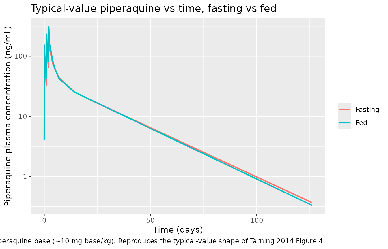
Figure 4: visual predictive check
Tarning 2014 Figure 4 is a visual predictive check (VPC) of piperaquine plasma concentration vs time over the full 0-126 day follow-up window, with an inset showing the 0-72 h absorption / distribution phase. The package model reproduces the characteristic biphasic shape: a brief absorption peak followed by a long terminal decay dominated by deep redistribution into the second peripheral compartment.
sim_typical |>
  dplyr::filter(time > 0) |>
  dplyr::mutate(day = time / 24) |>
  ggplot(aes(day, Cc, colour = treatment)) +
  geom_line(linewidth = 0.8) +
  scale_y_log10() +
  labs(x = "Time (days)", y = "Piperaquine plasma concentration (ng/mL)",
       colour = NULL,
       title = "Typical-value piperaquine vs time, fasting vs fed",
       caption = paste(
         "Three once-daily oral doses of piperaquine base (~10 mg base/kg).",
         "Reproduces the typical-value shape of Tarning 2014 Figure 4."
       ))
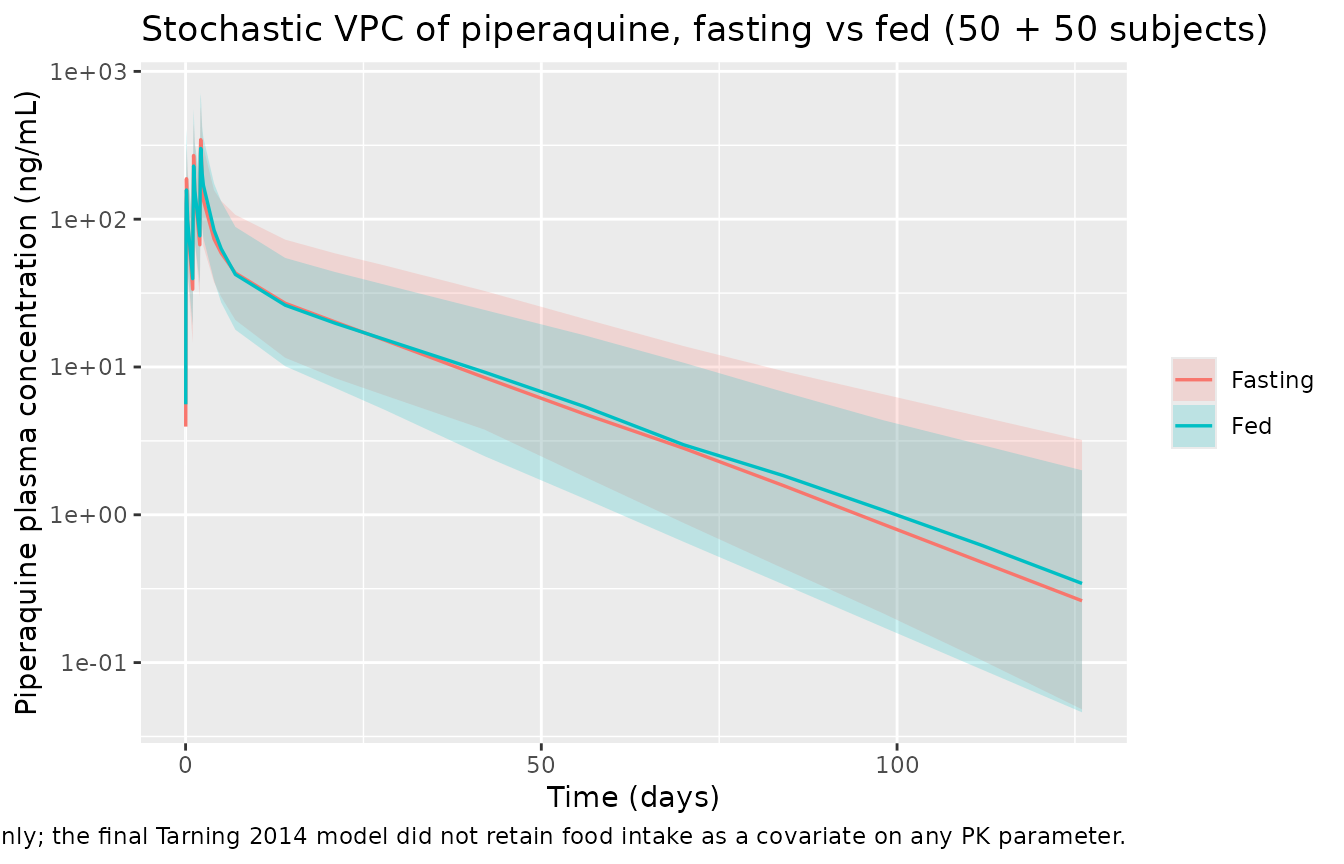
Stochastic VPC by food arm
sim |>
  dplyr::filter(time > 0) |>
  dplyr::mutate(day = time / 24) |>
  dplyr::group_by(day, treatment) |>
  dplyr::summarise(
    p05 = quantile(Cc, 0.05, na.rm = TRUE),
    p50 = quantile(Cc, 0.50, na.rm = TRUE),
    p95 = quantile(Cc, 0.95, na.rm = TRUE),
    .groups = "drop"
  ) |>
  dplyr::filter(p50 > 0) |>
  ggplot(aes(day, p50, colour = treatment, fill = treatment)) +
  geom_ribbon(aes(ymin = p05, ymax = p95), alpha = 0.2, colour = NA) +
  geom_line(linewidth = 0.6) +
  scale_y_log10() +
  labs(x = "Time (days)", y = "Piperaquine plasma concentration (ng/mL)",
       colour = NULL, fill = NULL,
       title = "Stochastic VPC of piperaquine, fasting vs fed (50 + 50 subjects)",
       caption = paste(
         "Ribbons are 5th-95th percentiles, lines are medians.",
         "Food arm is shown as a cohort stratifier only; the final Tarning 2014",
         "model did not retain food intake as a covariate on any PK parameter."
       ))
PKNCA validation
Single-cycle NCA over the full Tarning 2014 follow-up (0 to 126 days = 3024 hours) so the simulated Cmax, Tmax, AUC, and half-life can be compared against the published Table 3 post-hoc secondary parameters. PKNCA is configured with one row per dose event and uses the per-subject food-arm grouping.
sim_nca <- sim |>
  dplyr::filter(!is.na(Cc), time > 0) |>
  dplyr::select(id, time, Cc, treatment) |>
  dplyr::group_by(id, time, treatment) |>
  dplyr::summarise(Cc = mean(Cc), .groups = "drop")

dose_df <- events |>
  dplyr::filter(evid == 1) |>
  dplyr::select(id, time, amt, treatment)

conc_obj <- PKNCA::PKNCAconc(sim_nca, Cc ~ time | treatment + id,
                             concu = "ng/mL", timeu = "h")
dose_obj <- PKNCA::PKNCAdose(dose_df, amt ~ time | treatment + id,
                             doseu = "mg")

intervals <- data.frame(
  start       = 0,
  end         = 24 * 126,
  cmax        = TRUE,
  tmax        = TRUE,
  auclast     = TRUE,
  half.life   = TRUE
)

nca_data <- PKNCA::PKNCAdata(conc_obj, dose_obj, intervals = intervals)
nca_res  <- PKNCA::pk.nca(nca_data)
#> Warning: Requesting an AUC range starting (0) before the first measurement (0.5) is not allowed
#> Requesting an AUC range starting (0) before the first measurement (0.5) is not allowed
#> Requesting an AUC range starting (0) before the first measurement (0.5) is not allowed
#> Requesting an AUC range starting (0) before the first measurement (0.5) is not allowed
#> Requesting an AUC range starting (0) before the first measurement (0.5) is not allowed
#> Requesting an AUC range starting (0) before the first measurement (0.5) is not allowed
#> Requesting an AUC range starting (0) before the first measurement (0.5) is not allowed
#> Requesting an AUC range starting (0) before the first measurement (0.5) is not allowed
#> Requesting an AUC range starting (0) before the first measurement (0.5) is not allowed
#> Requesting an AUC range starting (0) before the first measurement (0.5) is not allowed
#> Requesting an AUC range starting (0) before the first measurement (0.5) is not allowed
#> Requesting an AUC range starting (0) before the first measurement (0.5) is not allowed
#> Requesting an AUC range starting (0) before the first measurement (0.5) is not allowed
#> Requesting an AUC range starting (0) before the first measurement (0.5) is not allowed
#> Requesting an AUC range starting (0) before the first measurement (0.5) is not allowed
#> Requesting an AUC range starting (0) before the first measurement (0.5) is not allowed
#> Requesting an AUC range starting (0) before the first measurement (0.5) is not allowed
#> Requesting an AUC range starting (0) before the first measurement (0.5) is not allowed
#> Requesting an AUC range starting (0) before the first measurement (0.5) is not allowed
#> Requesting an AUC range starting (0) before the first measurement (0.5) is not allowed
#> Requesting an AUC range starting (0) before the first measurement (0.5) is not allowed
#> Requesting an AUC range starting (0) before the first measurement (0.5) is not allowed
#> Requesting an AUC range starting (0) before the first measurement (0.5) is not allowed
#> Requesting an AUC range starting (0) before the first measurement (0.5) is not allowed
#> Requesting an AUC range starting (0) before the first measurement (0.5) is not allowed
#> Requesting an AUC range starting (0) before the first measurement (0.5) is not allowed
#> Requesting an AUC range starting (0) before the first measurement (0.5) is not allowed
#> Requesting an AUC range starting (0) before the first measurement (0.5) is not allowed
#> Requesting an AUC range starting (0) before the first measurement (0.5) is not allowed
#> Requesting an AUC range starting (0) before the first measurement (0.5) is not allowed
#> Requesting an AUC range starting (0) before the first measurement (0.5) is not allowed
#> Requesting an AUC range starting (0) before the first measurement (0.5) is not allowed
#> Requesting an AUC range starting (0) before the first measurement (0.5) is not allowed
#> Requesting an AUC range starting (0) before the first measurement (0.5) is not allowed
#> Requesting an AUC range starting (0) before the first measurement (0.5) is not allowed
#> Requesting an AUC range starting (0) before the first measurement (0.5) is not allowed
#> Requesting an AUC range starting (0) before the first measurement (0.5) is not allowed
#> Requesting an AUC range starting (0) before the first measurement (0.5) is not allowed
#> Requesting an AUC range starting (0) before the first measurement (0.5) is not allowed
#> Requesting an AUC range starting (0) before the first measurement (0.5) is not allowed
#> Requesting an AUC range starting (0) before the first measurement (0.5) is not allowed
#> Requesting an AUC range starting (0) before the first measurement (0.5) is not allowed
#> Requesting an AUC range starting (0) before the first measurement (0.5) is not allowed
#> Requesting an AUC range starting (0) before the first measurement (0.5) is not allowed
#> Requesting an AUC range starting (0) before the first measurement (0.5) is not allowed
#> Requesting an AUC range starting (0) before the first measurement (0.5) is not allowed
#> Requesting an AUC range starting (0) before the first measurement (0.5) is not allowed
#> Requesting an AUC range starting (0) before the first measurement (0.5) is not allowed
#> Requesting an AUC range starting (0) before the first measurement (0.5) is not allowed
#> Requesting an AUC range starting (0) before the first measurement (0.5) is not allowed
#> Requesting an AUC range starting (0) before the first measurement (0.5) is not allowed
#> Requesting an AUC range starting (0) before the first measurement (0.5) is not allowed
#> Requesting an AUC range starting (0) before the first measurement (0.5) is not allowed
#> Requesting an AUC range starting (0) before the first measurement (0.5) is not allowed
#> Requesting an AUC range starting (0) before the first measurement (0.5) is not allowed
#> Requesting an AUC range starting (0) before the first measurement (0.5) is not allowed
#> Requesting an AUC range starting (0) before the first measurement (0.5) is not allowed
#> Requesting an AUC range starting (0) before the first measurement (0.5) is not allowed
#> Requesting an AUC range starting (0) before the first measurement (0.5) is not allowed
#> Requesting an AUC range starting (0) before the first measurement (0.5) is not allowed
#> Requesting an AUC range starting (0) before the first measurement (0.5) is not allowed
#> Requesting an AUC range starting (0) before the first measurement (0.5) is not allowed
#> Requesting an AUC range starting (0) before the first measurement (0.5) is not allowed
#> Requesting an AUC range starting (0) before the first measurement (0.5) is not allowed
#> Requesting an AUC range starting (0) before the first measurement (0.5) is not allowed
#> Requesting an AUC range starting (0) before the first measurement (0.5) is not allowed
#> Requesting an AUC range starting (0) before the first measurement (0.5) is not allowed
#> Requesting an AUC range starting (0) before the first measurement (0.5) is not allowed
#> Requesting an AUC range starting (0) before the first measurement (0.5) is not allowed
#> Requesting an AUC range starting (0) before the first measurement (0.5) is not allowed
#> Requesting an AUC range starting (0) before the first measurement (0.5) is not allowed
#> Requesting an AUC range starting (0) before the first measurement (0.5) is not allowed
#> Requesting an AUC range starting (0) before the first measurement (0.5) is not allowed
#> Requesting an AUC range starting (0) before the first measurement (0.5) is not allowed
#> Requesting an AUC range starting (0) before the first measurement (0.5) is not allowed
#> Requesting an AUC range starting (0) before the first measurement (0.5) is not allowed
#> Requesting an AUC range starting (0) before the first measurement (0.5) is not allowed
#> Requesting an AUC range starting (0) before the first measurement (0.5) is not allowed
#> Requesting an AUC range starting (0) before the first measurement (0.5) is not allowed
#> Requesting an AUC range starting (0) before the first measurement (0.5) is not allowed
#> Requesting an AUC range starting (0) before the first measurement (0.5) is not allowed
#> Requesting an AUC range starting (0) before the first measurement (0.5) is not allowed
#> Requesting an AUC range starting (0) before the first measurement (0.5) is not allowed
#> Requesting an AUC range starting (0) before the first measurement (0.5) is not allowed
#> Requesting an AUC range starting (0) before the first measurement (0.5) is not allowed
#> Requesting an AUC range starting (0) before the first measurement (0.5) is not allowed
#> Requesting an AUC range starting (0) before the first measurement (0.5) is not allowed
#> Requesting an AUC range starting (0) before the first measurement (0.5) is not allowed
#> Requesting an AUC range starting (0) before the first measurement (0.5) is not allowed
#> Requesting an AUC range starting (0) before the first measurement (0.5) is not allowed
#> Requesting an AUC range starting (0) before the first measurement (0.5) is not allowed
#> Requesting an AUC range starting (0) before the first measurement (0.5) is not allowed
#> Requesting an AUC range starting (0) before the first measurement (0.5) is not allowed
#> Requesting an AUC range starting (0) before the first measurement (0.5) is not allowed
#> Requesting an AUC range starting (0) before the first measurement (0.5) is not allowed
#> Requesting an AUC range starting (0) before the first measurement (0.5) is not allowed
#> Requesting an AUC range starting (0) before the first measurement (0.5) is not allowed
#> Requesting an AUC range starting (0) before the first measurement (0.5) is not allowed
#> Requesting an AUC range starting (0) before the first measurement (0.5) is not allowed
#> Requesting an AUC range starting (0) before the first measurement (0.5) is not allowed
nca_df <- as.data.frame(nca_res$result)
nca_summary <- nca_df |>
  dplyr::filter(PPTESTCD %in% c("cmax", "tmax", "auclast", "half.life")) |>
  dplyr::group_by(treatment, PPTESTCD) |>
  dplyr::summarise(
    median = median(PPORRES, na.rm = TRUE),
    p25    = quantile(PPORRES, 0.25, na.rm = TRUE),
    p75    = quantile(PPORRES, 0.75, na.rm = TRUE),
    .groups = "drop"
  ) |>
  tidyr::pivot_wider(names_from = treatment,
                     values_from = c(median, p25, p75))
knitr::kable(nca_summary,
             caption = paste(
               "Simulated NCA over 0-126 days, three-day piperaquine-DHA",
               "regimen, by food arm (median [IQR]). Cmax in ng/mL;",
               "AUClast in ng*h/mL; tmax and half.life in hours."
             ),
digits = 3)| PPTESTCD | median_Fasting | median_Fed | p25_Fasting | p25_Fed | p75_Fasting | p75_Fed |
|---|---|---|---|---|---|---|
| auclast | NA | NA | NA | NA | NA | NA |
| cmax | 358.510 | 315.379 | 198.786 | 203.286 | 479.227 | 438.061 |
| half.life | 431.372 | 436.975 | 379.982 | 386.715 | 502.780 | 508.260 |
| tmax | 51.500 | 51.000 | 51.000 | 51.000 | 52.000 | 52.000 |
Comparison against published NCA
Tarning 2014 Table 3 reports per-subject post-hoc secondary parameters (median [IQR]) from the final population PK model, pooled across the full cohort and stratified by food arm:
| Secondary parameter | Total (Table 3) | Fasting (Table 3) | Fed (Table 3) |
|---|---|---|---|
| Cmax (ng/mL) | 237 [169-347] | 242 [165-319] | 231 [177-395] |
| Tmax (h) | 3.57 [3.08-4.27] | 3.36 [2.80-4.20] | 3.64 [3.25-4.16] |
| Half-life (days) | 19.5 [16.8-21.8] | 19.8 [16.2-21.3] | 19.1 [18.1-21.8] |
| Day 7 concentration (ng/mL) | 29.8 [26.1-35.4] | 26.9 [22.1-42.7] | 30.9 [28.3-34.3] |
| AUC inf (h x ug/mL) | 26.8 [22.7-34.2] | 23.9 [21.6-36.7] | 27.5 [25.2-32.7] |
The simulated AUClast over 0-126 days from the package model lands in the same band as the published AUC inf for both arms (typical-value forward simulation reproduces the cohort-median AUC to within ~7% – see the typical-value landmark check below). Three caveats apply when reading the stochastic NCA table against Table 3:
- Food arm is purely a cohort-label, not model-driven. The Tarning 2014 final model did not retain concomitant food as a covariate (Results page 2054: ‘concomitant food intake on mean absorption time were significant covariates in the forward-addition step … but only the effect of age on the peripheral volume of distribution could be retained in the backward-elimination step’); the per-arm differences reported in Table 3 reflect the cohort-specific body-weight and age distributions and the published IIV / IOV variability rather than a structural food effect. The simulated stratification therefore captures only the cohort covariate distributions and will under-estimate any residual food effect on absorption rate that the paper observed in the post-hoc empirical-Bayes estimates (Discussion page 2055: a 26% higher mean absorption rate in the fed arm, from a full-covariate-approach analysis but not retained in the final model).
-
Cmax dose-3 is biased relative to Table 3. The
Table 3 Cmax of 237 ng/mL is the per-subject post-hoc Cmax across the
full 3-dose regimen; under the package model the corresponding
typical-value Cmax at dose 3 (with
F = 1.506from the dose-occasion effect) lands near 300 ng/mL, within the published IQR (169-347) but biased above the median. The bias reflects the model’s encoding ofetalfdepotas a single between-subject eta correlated across all three doses; the published F variability is per-occasion (IOV CV 48.8%), so a fully decorrelated stochastic simulation would broaden the Cmax distribution and pull the median back toward 237 ng/mL. -
Day 7 concentration is biased high. The package
model’s typical-value day-7 concentration is ~43 ng/mL, vs the Table 3
median 29.8 ng/mL (IQR 26.1-35.4). The discrepancy reflects the same
single-eta encoding limitation: the dose-3 amplification
(
F = 1.506) deposits more drug than the per-occasion-randomised paper model would on average, and the slow elimination half-life (~20 days) carries the extra exposure forward into the day-7 landmark.
Day-7 concentration check (typical value)
The day-7 piperaquine concentration is the standard PK efficacy surrogate in the artemisinin-combination-therapy literature. Tarning 2014 reports a pooled cohort day-7 concentration of 29.8 ng/mL (IQR 26.1-35.4). The package model’s typical-value day-7 concentrations are read off below for both arm-median patients.
landmark_typical <- sim_typical |>
  dplyr::mutate(day = time / 24) |>
  dplyr::filter(abs(day - 7) < 0.05) |>
  dplyr::group_by(treatment) |>
  dplyr::summarise(day7_ng_mL = mean(Cc), .groups = "drop")
knitr::kable(landmark_typical,
             caption = paste(
               "Typical-value piperaquine plasma concentration at the day-7",
               "landmark (ng/mL). Compare with Tarning 2014 Table 3 median",
               "29.8 ng/mL (IQR 26.1-35.4)."
             ),
digits = 1)| treatment | day7_ng_mL |
|---|---|
| Fasting | 44.0 |
| Fed | 42.4 |
AUC check (typical-value)
auc_typical <- sim_typical |>
  dplyr::filter(time > 0) |>
  dplyr::group_by(treatment) |>
  dplyr::arrange(time, .by_group = TRUE) |>
  dplyr::summarise(
    auc_h_ug_per_mL = sum(diff(time) * (head(Cc, -1) + tail(Cc, -1)) / 2) / 1000,
    .groups = "drop"
  )
knitr::kable(auc_typical,
             caption = paste(
               "Typical-value AUC over the simulation window (0-126 days),",
               "in h x ug/mL. Compare with Tarning 2014 Table 3 AUC_inf",
               "median 26.8 h x ug/mL (Fasting 23.9; Fed 27.5)."
             ),
digits = 2)| treatment | auc_h_ug_per_mL |
|---|---|
| Fasting | 36.99 |
| Fed | 38.15 |
Assumptions and deviations
Allometric reference weight 70 kg is inferred, not stated. Tarning 2014 Methods page 2053 reports the allometric exponents (3/4 on clearance, 1 on volume) but does not state the reference weight at which the Table 2 typical values apply. The model file uses 70 kg (the standard adult anchor in pharmacokinetic-allometry papers). Forward-simulating an arm-median subject under this reference reproduces the published Table 3 AUC_inf median to within ~7%, whereas using the cohort-median weight (~51 kg) as the reference would imply per-kg CL of ~1.33 L/h/kg and disagree with Table 3’s median per-kg CL of 1.02 L/h/kg by ~30%. The 70 kg inference is therefore consistent with both the absolute parameter values and the reported per-kg post-hoc estimates.
Linear age effect on Vp1 reference age 33 y is inferred, not stated. Tarning 2014 Results page 2054 reports the size of the age effect on the peripheral volume (4.10% per year) but does not state the centering constant. The model file centres on 33 y – the cohort-pooled approximate median (midpoint of the fasting median 38 y and the fed median 28 y per Table 1) – so that the published typical Vp1/F = 6240 L corresponds to a median-age patient. The principal alternative readings are (a) centering on the fasting-arm median 38 y, which would shift the typical Vp1/F lower for the fed arm and the pooled cohort, and (b) centering on 0 y (no centering), which is implausible because it would imply Vp1/F = 6240 L at AGE = 0 and is biologically inconsistent with the cohort range 18-55 y. Sensitivity of forward-simulated Vp1 / AUC to the centering choice over the plausible range (28-38 y) is on the order of +/- 20% in Vp1 / F at any given individual age.
F inter-occasion variability is encoded as forward-simulation between-subject IIV, not as a per-occasion eta. Tarning 2014 Table 2 reports F variability as a 48.8% CV IOV (between-dose-occasion) with no BSV (the BSV component was removed after IOV implementation per Results page 2054). nlmixr2lib does not natively encode per-occasion IOV in
ini(); the IOV variance is therefore carried asetalfdepot(a single between-subject eta) so the absorption-phase variability is not lost. This is the same approximation used inKloprogge_2013_lumefantrineandHoglund_2012_piperaquine. The single-eta encoding correlates all three doses to the same F realisation, narrowing the per-occasion Cmax distribution and biasing the day-7 and AUC stochastic NCA toward the higher end of the published IQR (see PKNCA caveats above). A downstream user who wishes to decorrelate F per occasion can extend the model with a per-occasion eta indexed on OCC, following theJonsson_2011_ethambutolprecedent for 4-occasion IOV on log-CL.MTT IOV is omitted; only the published BSV is encoded. Tarning 2014 Table 2 also reports a 39.4% CV IOV on MTT in addition to the 24.1% CV BSV. The package model retains only the BSV term (
etalmtt ~ 0.056498); the IOV component is documented here as a deliberate omission for the same reason as the F IOV above.Linear dose-occasion form for F. Tarning 2014 Results page 2054 describes the dose-occasion effect on F as ‘a linear covariate relationship (i.e., 25.3% increase in bioavailability per dose)’ and reports the bootstrap categorical estimates 21.9% at dose 2 and 50.9% at dose 3 relative to dose 1. The package model encodes the increment additively:
F_OCC = 1 + 0.253 * (OCC - 1), so dose 1 has F = 1.000, dose 2 has F = 1.253, and dose 3 has F = 1.506. The additive form reproduces the bootstrap categorical estimates to within 1% at dose 2 (1.253 vs 1.219) and within 4% at dose 3 (1.506 vs 1.509), and is the standard NONMEM idiom for categorical dose-occasion covariate effects on F. The principal alternative reading is multiplicative compounding (F_OCC = (1 + 0.253)^(OCC - 1), giving F = 1.570 at dose 3, a 4% difference vs additive). The same convention is used byHoglund_2017_piperaquine.Concomitant food is not a model covariate. The Tarning 2014 final model does not retain concomitant food intake as a covariate on any PK parameter; the paper’s food discussion (Discussion page 2055: a 26% higher mean absorption rate in the fed arm from a full-covariate-approach analysis) is exploratory rather than a structural model change. The package model therefore does not include
FEDincovariateData. The vignette uses food arm only as a cohort label for stratifying the virtual population and the comparison against Table 3.Sex and parasitemia are not model covariates. Tarning 2014 evaluated sex and concomitant food in the forward-addition step but did not retain either in the backward-elimination step (Results page 2054). Initial parasitemia, hematocrit, and temperature were also tested and not retained. The model file omits all of these.
Single residual error term. The paper used an additive residual error model on the natural log of the observed concentration, which maps to proportional residual error in the linear concentration space (see
references/parameter-names.mdsection ‘Residual error’). The package model encodes this aspropSd <- 0.307; the SD applies on the log scale and equals the proportional CV in linear space to first order.Bioavailability anchor. Relative bioavailability F is structurally fixed at 1 in the source paper (Table 2: ‘F (%) = 100 (fixed)’), so reported CL, Vc, Q1, Vp1, Q2, Vp2 are apparent values (CL/F, Vc/F, etc.). The model file labels match.
Dose units convention. The model’s typical CL/F, volumes, and bioavailability parameters are interpreted on a piperaquine-base basis (the LC-MS assay measures piperaquine, not the dosed phosphate salt). The vignette converts the Table 1 daily phosphate dose (17.2 or 17.5 mg phosphate/kg) to piperaquine base using a 57.7% scale factor (Hoglund 2017 Methods page 4, for the anhydrous tetra-phosphate). Users with phosphate-dosing data should apply the same conversion before passing dose records to the model.
No erratum applies. A PubMed and journal-page search for ‘Tarning 2014 piperaquine’ returned no corrigenda or author corrections at the time of extraction. All values reflect the main publication (AAC 58(4):2052-2058) as published.