d-Tubocurarine (Sheiner 1979)
Source:vignettes/articles/Sheiner_1979_tubocurarine.Rmd
Sheiner_1979_tubocurarine.RmdModel and source
- Citation: Sheiner LB, Stanski DR, Vozeh S, Miller RD, Ham J. Simultaneous modeling of pharmacokinetics and pharmacodynamics: application to d-tubocurarine. Clin Pharmacol Ther. 1979;25(3):358-371. doi:10.1002/cpt1979253358. Read from the full facsimile reprint bundled with Karlsson MO, In the cradle of pharmacometric methodology: introducing population PKPD modeling, simultaneous analysis and the effect-compartment model. Commentary on Sheiner et al. Clin Pharmacol Ther. 2025;117(6):1516-1532. doi:10.1002/cpt.3663 (PMC12087688), pages 1519-1532.
- Description: Two-compartment IV population PK linked to a hypothetical effect compartment and a sigmoid Emax pharmacodynamic model for d-tubocurarine (dTC) neuromuscular blockade in 20 adults undergoing elective surgery, 10 with normal renal function and 10 with chronic end-stage renal failure awaiting renal transplantation (Sheiner 1979, group 3). This is the founding effect-compartment paper: plasma concentration and effect (degree of thumb-adduction paralysis, 0 = none to 1 = complete) were fitted simultaneously by nonlinear mixed effects, and the effect compartment is parameterised so that its concentration is the equivalent steady-state plasma concentration Cpss. Renal failure is encoded exactly as the paper’s baseline model does, as the absence of the renal elimination arm of clearance, with no other structural difference between the two groups.
- Article: https://doi.org/10.1002/cpt1979253358
- Facsimile reprint used as the source: https://doi.org/10.1002/cpt.3663 (PMC12087688, pages 1519-1532)
This is the paper that introduced the hypothetical effect-compartment model, simultaneous PK/PD fitting, and (with Sheiner, Rosenberg and Marathe 1977) the use of nonlinear mixed effects in pharmacometrics. The 2025 Clinical Pharmacology & Therapeutics “Historical Perspective” commentary by Karlsson reprints the 1979 article in full as a facsimile; that reprint is the source document read for this extraction.
Two data sets are analysed in the paper. Group 1 (7 patients, dual infusion) was fitted subject-by-subject with nonlinear least squares. Group 3 (20 patients, single IV bolus, 10 with normal renal function and 10 with chronic end-stage renal failure) was fitted by nonlinear mixed effects with plasma and effect data analysed simultaneously. The packaged model is the group 3 fit, because it is the only one of the two for which a complete, mutually consistent PK and PD parameterisation can be recovered from the paper (see Assumptions and deviations).
Population
Group 3 consists of 20 adults undergoing elective surgery: 10 with normal serum creatinine and 10 with chronic end-stage renal failure undergoing renal transplantation. The renal failure patients were anaemic (haemoglobin 6.8 +/- 1.5 g/100 mL) and had markedly elevated serum creatinine (10.1 +/- 2.3 mg/100 mL) in spite of recent dialysis; all were studied prior to insertion of the transplant kidney (p. 362). Anaesthesia was induced with nitrous oxide:oxygen and halothane with the trachea intubated without drugs, and maintained with nitrous oxide (60%):oxygen and halothane at an end-tidal concentration of 0.45 to 0.8%.
Twenty minutes after induction each subject received a single IV bolus of d-tubocurarine (dTC): within each of the normal and renal failure groups, 5 subjects received 0.3 mg/kg and 5 received 0.5 mg/kg. Blood samples were drawn at 3, 15, 30, 45, 60, 90 and 120 min, with additional 150 and 180 min samples after the 0.5 mg/kg dose, giving 7 to 9 data points per patient. dTC was assayed by radioimmunoassay (assay CV 8%, lower limit of sensitivity 0.05 ug/mL). Effect was the force of thumb adduction after supramaximal ulnar nerve stimulation, expressed as the degree of paralysis from 0 (none) to 1.0 (complete). Neither ages nor body weights are reported for group 3.
The same information is available programmatically via
readModelDb("Sheiner_1979_tubocurarine")()$population.
Source trace
| Equation / parameter | Value | Source location |
|---|---|---|
| Two-compartment mammillary disposition | n/a | Eq. 3 and p. 362 Data analysis (“fitted to a biexponential equation interpreted as a 2-compartment mammillary model”) |
Effect compartment
d/dt(effect) <- ke0 * (Cc - effect)
|
n/a | Eq. 2 rescaled by Eq. 7 (p. 360-361); k1e cancels out
of Eq. 7 |
Sigmoid Emax
paralysis <- emax * effect^hill / (ec50^hill + effect^hill)
|
n/a | Eq. 1 and Eq. 8 (p. 358, 361) |
| Renal failure = loss of the renal clearance arm only | n/a | p. 363 (“the only distinction between N and RF patients was the absence of a renal elimination rate constant in the RF patients”) |
lvc (Vc) |
5.443 L / 70 kg (77.8 mL/kg) | Fig. 3 (p. 364), digitised - see below |
lvp (Vp) |
11.87 L / 70 kg (169.5 mL/kg) | Fig. 3 (p. 364), digitised |
lq (Q) |
0.3654 L/min / 70 kg (5.22 mL/min/kg) | Fig. 3 (p. 364), digitised |
lcl_nonren |
0.1037 L/min / 70 kg (1.48 mL/min/kg) | Fig. 3 (p. 364), digitised |
lcl_renal |
0.06639 L/min / 70 kg (0.95 mL/min/kg) | Fig. 3 (p. 364), digitised |
e_wt_cl, e_wt_vc
|
1 (fixed) | Encoding of the paper’s mg/kg dosing (p. 362); not fitted by the paper |
lke0 (keo) |
0.16 /min | Table II (p. 365), group 3 column |
lhill (gamma) |
2.30 | Table II (p. 365), group 3 column |
lec50 (Cpss(50)) |
0.38 ug/mL | Table II (p. 365), group 3 column |
lemax |
1 (fixed) | Eq. 1 / Eq. 8: E is the fraction of maximal response (p. 362) |
The paper states plainly (p. 365) that “the pharmacokinetic parameter estimates are not presented because they are not of central concern to this paper”. They are nevertheless published graphically: the heavy solid lines of Fig. 3 are the estimated mean population concentration-time response, one per dose and per renal group. The five disposition parameters above were recovered by digitising all four of those curves at the nine sampling times (36 points) and fitting a single two-compartment IV bolus model constrained so that renal failure removes only the renal arm of clearance - the paper’s own baseline structure. No parameter was tuned against any effect-time observation.
Digitised source figures
The digitised values below are the raw material for the validation
that follows. Fig. 3 values are plasma dTC in ug/mL; Fig. 4 values are
the fraction of maximal paralysis. NA marks a sampling time
at which the population marker is obscured by overlapping individual
profiles.
sample_times <- c(3, 15, 30, 45, 60, 90, 120, 150, 180)

digitised <- tibble::tibble(
  arm = rep(c("Normal, 0.5 mg/kg", "Normal, 0.3 mg/kg",
              "Renal failure, 0.5 mg/kg", "Renal failure, 0.3 mg/kg"),
            each = length(sample_times)),
  time = rep(sample_times, times = 4),
  fig3_conc = c(
    4.610, 1.955, 1.173, 0.919, 0.809, 0.632, 0.502, 0.403, 0.317,
    2.872, 1.170, 0.685, 0.549, 0.483, 0.386, 0.297, 0.233, 0.187,
    5.099, 2.426, 1.498, 1.250, 1.158, 0.996, 0.835, 0.702, 0.594,
    3.099, 1.402, 0.889, 0.755, 0.676, 0.573, 0.483, 0.417, 0.352),
  fig4_paralysis = c(
    0.995, 0.995, 0.968, 0.945, 0.905, 0.837, 0.742, 0.628, 0.484,
    0.955,    NA, 0.910, 0.806, 0.722, 0.613, 0.475, 0.347, 0.226,
    1.002, 0.989, 0.970, 0.969, 0.935, 0.921, 0.894, 0.859, 0.793,
    0.945,    NA, 0.914, 0.891, 0.839, 0.790, 0.711, 0.617, 0.543)
)
A first, source-independent check on the digitisation: dTC disposition is assumed linear, so within a renal group the 0.5 and 0.3 mg/kg population curves must be exact multiples of one another with ratio 5/3.
digitised |>
  tidyr::separate_wider_delim(arm, ", ", names = c("group", "dose")) |>
  select(group, dose, time, fig3_conc) |>
  tidyr::pivot_wider(names_from = dose, values_from = fig3_conc) |>
  mutate(ratio = `0.5 mg/kg` / `0.3 mg/kg`) |>
  group_by(group) |>
  summarise(
    `Mean ratio (expected 1.667)` = mean(ratio),
    `Max absolute deviation (%)` = max(abs(100 * (ratio / (5 / 3) - 1))),
    .groups = "drop"
  ) |>
  rename("Renal group" = group) |>
  knitr::kable(digits = 2,
caption = "Linearity check on the digitised Fig. 3 population curves.")| Renal group | Mean ratio (expected 1.667) | Max absolute deviation (%) |
|---|---|---|
| Normal | 1.68 | 3.78 |
| Renal failure | 1.70 | 4.29 |
Virtual cohort
The packaged model is a typical-value (population mean)
model: the group 3 analysis did estimate interindividual
variability, but no variance component is tabulated anywhere in the
paper and none may be invented, so no eta and no
residual-error term is encoded. Simulating a stochastic cohort would
therefore add nothing - every subject would be identical. The cohort
below is instead one typical subject per published arm, which is exactly
what the heavy solid lines of Fig. 3 and Fig. 4 depict.
Body weight is fixed at 70 kg. Because both clearance and volume terms scale linearly with weight, the predicted concentration after a mg/kg dose is weight invariant, so this choice does not affect any result below.
WT_KG <- 70

arms <- tibble::tribble(
  ~arm,                       ~dose_mgkg, ~RENALIMP_SEV,
  "Normal, 0.3 mg/kg",               0.3,             0,
  "Normal, 0.5 mg/kg",               0.5,             0,
  "Renal failure, 0.3 mg/kg",        0.3,             1,
  "Renal failure, 0.5 mg/kg",        0.5,             1
) |>
  mutate(id = row_number())

obs_grid <- seq(0, 180, by = 0.5)

events <-
  arms |>
  rowwise() |>
  reframe(
    id = id,
    arm = arm,
    RENALIMP_SEV = RENALIMP_SEV,
    WT = WT_KG,
    time = c(0, obs_grid),
    evid = c(1L, rep(0L, length(obs_grid))),
    amt = c(dose_mgkg * WT_KG, rep(NA_real_, length(obs_grid))),
    cmt = "central"
  ) |>
  arrange(id, time, desc(evid))

stopifnot(nrow(arms) <= 200L)
Observation rows point at the ODE state central, not at
the algebraic observables Cc / paralysis;
rxode2 returns every algebraic observable as an output column
regardless.
Simulation
mod <- readModelDb("Sheiner_1979_tubocurarine")
sim <- rxode2::rxSolve(
  mod,
  events = events,
  keep = c("arm", "RENALIMP_SEV"),
  returnType = "data.frame"
)
Replicate published figures
ggplot(sim, aes(time, Cc, colour = arm)) +
  geom_line(linewidth = 0.8) +
  geom_point(
    data = digitised, aes(time, fig3_conc, colour = arm),
    inherit.aes = FALSE, size = 2, shape = 21, fill = "white"
  ) +
  scale_y_log10(limits = c(0.1, 8)) +
  labs(
    x = "Time (min)", y = "Plasma d-tubocurarine (ug/mL)", colour = NULL,
    title = "Figure 3 - population mean plasma concentration",
    caption = "Lines: packaged model. Points: digitised heavy lines of Fig. 3 of Sheiner 1979."
  ) +
  theme(legend.position = "bottom")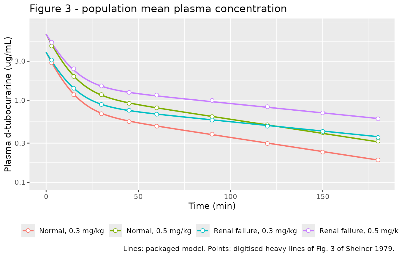
Replicates Figure 3 of Sheiner 1979.
ggplot(sim, aes(time, paralysis, colour = arm)) +
  geom_line(linewidth = 0.8) +
  geom_point(
    data = digitised, aes(time, fig4_paralysis, colour = arm),
    inherit.aes = FALSE, size = 2, shape = 21, fill = "white"
  ) +
  coord_cartesian(ylim = c(0, 1)) +
  labs(
    x = "Time (min)", y = "Effect (fraction of maximal paralysis)", colour = NULL,
    title = "Figure 4 - population mean neuromuscular blockade",
    caption = "Lines: packaged model. Points: digitised heavy lines of Fig. 4 of Sheiner 1979."
  ) +
  theme(legend.position = "bottom")
#> Warning: Removed 2 rows containing missing values or values outside the scale range
#> (`geom_point()`).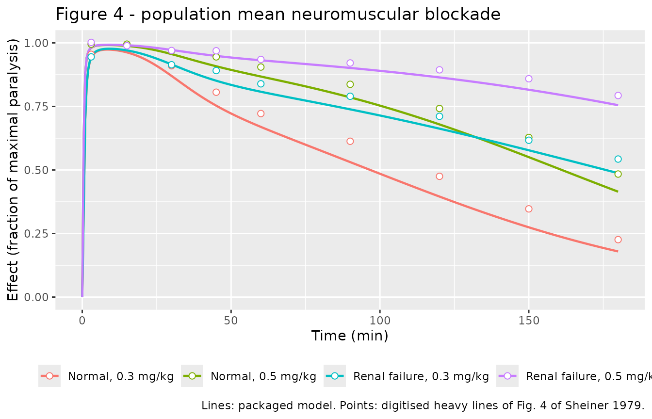
Replicates Figure 4 of Sheiner 1979.
agreement <-
  sim |>
  filter(time %in% sample_times) |>
  select(arm, time, Cc, effect, paralysis) |>
  left_join(digitised, by = c("arm", "time")) |>
  mutate(
    conc_pct_diff = 100 * (Cc / fig3_conc - 1),
    paralysis_diff = paralysis - fig4_paralysis
  )

agreement |>
  group_by(arm) |>
  summarise(
    `Median |% diff|, Cc vs Fig. 3` = median(abs(conc_pct_diff)),
    `Max |% diff|, Cc vs Fig. 3` = max(abs(conc_pct_diff)),
    `Median |diff|, effect vs Fig. 4` = median(abs(paralysis_diff), na.rm = TRUE),
    `Max |diff|, effect vs Fig. 4` = max(abs(paralysis_diff), na.rm = TRUE),
    .groups = "drop"
  ) |>
  rename("Arm" = arm) |>
  knitr::kable(digits = c(0, 2, 2, 3, 3),
caption = "Agreement of the packaged model with the digitised population curves.")| Arm | Median |% diff|, Cc vs Fig. 3 | Max |% diff|, Cc vs Fig. 3 | Median |diff|, effect vs Fig. 4 | Max |diff|, effect vs Fig. 4 |
|---|---|---|---|---|
| Normal, 0.3 mg/kg | 1.29 | 1.76 | 0.053 | 0.082 |
| Normal, 0.5 mg/kg | 1.34 | 4.87 | 0.037 | 0.078 |
| Renal failure, 0.3 mg/kg | 0.70 | 2.92 | 0.040 | 0.055 |
| Renal failure, 0.5 mg/kg | 1.63 | 3.53 | 0.020 | 0.043 |
The concentration-time reproduction is essentially exact, which it must be - those four curves are what the disposition parameters were recovered from. The effect-time reproduction is an independent check: nothing in Fig. 4 was used to derive any packaged value, and the three PD parameters come from Table II. The model tracks the shape and the dose- and renal-group separation of Fig. 4 closely but sits systematically a little below it; that offset is quantified and explained in the next section.
Internal consistency of the effect model
Two closed-form checks recover published quantities from the packaged parameters without any simulation.
ini_vals <- rxode2::rxode(mod)$theta

tibble::tribble(
  ~Quantity, ~`Packaged model`, ~`Sheiner 1979`, ~Source,
  "Effect-compartment half-life (min)",
  log(2) / exp(ini_vals[["lke0"]]), 4.33, "Table II, group 3",
  "Renal arm as a fraction of total clearance in normals (%)",
  100 * exp(ini_vals[["lcl_renal"]]) /
    (exp(ini_vals[["lcl_renal"]]) + exp(ini_vals[["lcl_nonren"]])),
  NA_real_, "Not reported; derived from Fig. 3"
) |>
  knitr::kable(digits = 2,
caption = "Closed-form checks against tabulated values.")| Quantity | Packaged model | Sheiner 1979 | Source |
|---|---|---|---|
| Effect-compartment half-life (min) | 4.33 | 4.33 | Table II, group 3 |
| Renal arm as a fraction of total clearance in normals (%) | 39.03 | NA | Not reported; derived from Fig. 3 |
Figure 4 also carries its own estimate of the Hill coefficient,
independent of Table II. Within a renal group the two doses share
gamma and Cpss(50) and differ only by a factor
5/3 in effect-site concentration, so the odds ratio of the two published
effect curves is (5/3)^gamma at every time. Times at which
either curve is above 0.95 are excluded: near-complete paralysis is
uninformative about the concentration-effect relationship, as the paper
itself notes (“responses close to maximal … do not contribute much, if
any, information to the pharmacodynamic parameter estimates”, p. 368),
and the odds ratio there is dominated by the last digitised decimal.
digitised |>
  filter(!is.na(fig4_paralysis)) |>
  tidyr::separate_wider_delim(arm, ", ", names = c("group", "dose")) |>
  select(group, dose, time, fig4_paralysis) |>
  tidyr::pivot_wider(names_from = dose, values_from = fig4_paralysis) |>
  filter(!is.na(`0.5 mg/kg`), !is.na(`0.3 mg/kg`),
         `0.5 mg/kg` <= 0.95, `0.3 mg/kg` <= 0.95) |>
  mutate(
    odds_hi = `0.5 mg/kg` / (1 - `0.5 mg/kg`),
    odds_lo = `0.3 mg/kg` / (1 - `0.3 mg/kg`),
    gamma_implied = log(odds_hi / odds_lo) / log(5 / 3)
  ) |>
  filter(is.finite(gamma_implied)) |>
  group_by(group) |>
  summarise(
    `Informative times (n)` = dplyr::n(),
    `Implied gamma (mean)` = mean(gamma_implied),
    `Implied gamma (SD)` = sd(gamma_implied),
    `Tabulated gamma` = 2.30,
    .groups = "drop"
  ) |>
  rename("Renal group" = group) |>
  knitr::kable(digits = 3,
caption = "Hill coefficient recovered from the dose pair of Fig. 4 vs Table II.")| Renal group | Informative times (n) | Implied gamma (mean) | Implied gamma (SD) | Tabulated gamma |
|---|---|---|---|---|
| Normal | 6 | 2.406 | 0.212 | 2.3 |
| Renal failure | 5 | 2.302 | 0.229 | 2.3 |
Figure 4 independently reproduces the tabulated gamma of
2.30. Inverting the same sigmoid for Cpss(50), using the
simulated effect-site concentration, isolates where the residual
disagreement with Fig. 4 lives.
agreement |>
  filter(!is.na(fig4_paralysis), fig4_paralysis < 0.99, effect > 0) |>
  mutate(
    ec50_implied =
      effect / (fig4_paralysis / (1 - fig4_paralysis))^(1 / exp(ini_vals[["lhill"]]))
  ) |>
  summarise(
    `Cpss(50) implied by Figs. 3 + 4 (ug/mL)` = mean(ec50_implied),
    `SD` = sd(ec50_implied),
    `Tabulated Cpss(50) (ug/mL)` = 0.38
  ) |>
  knitr::kable(digits = 3,
caption = "Cpss(50) back-solved from the two published figures vs Table II.")| Cpss(50) implied by Figs. 3 + 4 (ug/mL) | SD | Tabulated Cpss(50) (ug/mL) |
|---|---|---|
| 0.341 | 0.024 | 0.38 |
The two figures are mutually consistent to within a few percent but
imply a Cpss(50) about 10% below the 0.38 ug/mL of Table
II. Table II is the authoritative, tabulated value and is what the model
carries; the residual offset against Fig. 4 seen above is exactly this
discrepancy propagated through the sigmoid. No parameter was
adjusted to close it. Given the source is a 47-year-old scanned
figure, part of the gap is digitisation error; the remainder is a
table-versus-figure inconsistency in the original publication.
PKNCA validation
sim_nca <-
  sim |>
  dplyr::filter(!is.na(Cc)) |>
  dplyr::select(id, time, Cc, arm)

conc_obj <- PKNCA::PKNCAconc(as.data.frame(sim_nca), Cc ~ time | arm + id)

dose_df <-
  events |>
  dplyr::filter(evid == 1L) |>
  dplyr::select(id, time, amt, arm)

dose_obj <- PKNCA::PKNCAdose(as.data.frame(dose_df), amt ~ time | arm + id)

intervals <- data.frame(
  start = 0, end = Inf,
  cmax = TRUE, tmax = TRUE, aucinf.obs = TRUE, half.life = TRUE, cl.obs = TRUE
)

nca_res <- suppressWarnings(
  PKNCA::pk.nca(PKNCA::PKNCAdata(conc_obj, dose_obj, intervals = intervals))
)

nca_wide <-
  as.data.frame(nca_res$result) |>
  dplyr::select(arm, PPTESTCD, PPORRES) |>
  tidyr::pivot_wider(names_from = PPTESTCD, values_from = PPORRES)
Because a bolus dose is given at time 0, the time-zero concentration returned by the solver is the post-dose C0, so no defensive time-zero record is added.
Comparison against closed-form predictions
Sheiner 1979 reports no noncompartmental parameters at all, so there
is no published NCA table to compare against. The comparison below is
instead against the values implied in closed form by the packaged
ini() block: total clearance is
cl_nonren + cl_renal * (1 - RENALIMP_SEV), the terminal
half-life is log(2) divided by the smaller eigenvalue of
the two-compartment system, and C0 is dose divided by Vc. Disagreement
here would indicate a coding or solver problem rather than a source
discrepancy.
theta <- rxode2::rxode(mod)$theta
vc <- exp(theta[["lvc"]]); vp <- exp(theta[["lvp"]]); q <- exp(theta[["lq"]])

terminal_half_life <- function(cl) {
  k10 <- cl / vc; k12 <- q / vc; k21 <- q / vp
  s <- k10 + k12 + k21
  beta <- (s - sqrt(s^2 - 4 * k10 * k21)) / 2
  log(2) / beta
}

published_ref <-
  arms |>
  mutate(
    cl = exp(theta[["lcl_nonren"]]) + exp(theta[["lcl_renal"]]) * (1 - RENALIMP_SEV),
    cmax = dose_mgkg * WT_KG / vc,
    tmax = 0,
    aucinf.obs = dose_mgkg * WT_KG / cl,
    half.life = vapply(cl, terminal_half_life, numeric(1)),
    cl.obs = cl
  ) |>
  select(arm, cmax, tmax, aucinf.obs, half.life, cl.obs)

cmp <- nlmixr2lib::ncaComparisonTable(
  simulated = nca_res,
  reference = published_ref,
  by = "arm",
  units = c(cmax = "ug/mL", aucinf.obs = "ug*min/mL",
            tmax = "min", half.life = "min", cl.obs = "L/min"),
  tolerance_pct = 20
)

knitr::kable(
  cmp,
  caption = "Simulated NCA vs closed-form prediction from the packaged parameters. * differs by >20%.",
  align = c("l", "l", "r", "r", "r")
)| NCA parameter | arm | Reference | Simulated | % diff |
|---|---|---|---|---|
| Cmax (ug/mL) | Normal, 0.3 mg/kg | 3.86 | 3.86 | +0.0% |
| Cmax (ug/mL) | Normal, 0.5 mg/kg | 6.43 | 6.43 | +0.0% |
| Cmax (ug/mL) | Renal failure, 0.3 mg/kg | 3.86 | 3.86 | +0.0% |
| Cmax (ug/mL) | Renal failure, 0.5 mg/kg | 6.43 | 6.43 | +0.0% |
| Tmax (min) | Normal, 0.3 mg/kg | 0 | 0 | — |
| Tmax (min) | Normal, 0.5 mg/kg | 0 | 0 | — |
| Tmax (min) | Renal failure, 0.3 mg/kg | 0 | 0 | — |
| Tmax (min) | Renal failure, 0.5 mg/kg | 0 | 0 | — |
| AUC0-∞ (obs) (ug*min/mL) | Normal, 0.3 mg/kg | 123 | 123 | -0.1% |
| AUC0-∞ (obs) (ug*min/mL) | Normal, 0.5 mg/kg | 206 | 206 | -0.1% |
| AUC0-∞ (obs) (ug*min/mL) | Renal failure, 0.3 mg/kg | 203 | 202 | -0.2% |
| AUC0-∞ (obs) (ug*min/mL) | Renal failure, 0.5 mg/kg | 338 | 337 | -0.2% |
| t½ (min) | Normal, 0.3 mg/kg | 87.4 | 86.7 | -0.7% |
| t½ (min) | Normal, 0.5 mg/kg | 87.4 | 86.7 | -0.7% |
| t½ (min) | Renal failure, 0.3 mg/kg | 132 | 131 | -0.7% |
| t½ (min) | Renal failure, 0.5 mg/kg | 132 | 131 | -0.7% |
| CL/F (L/min) | Normal, 0.3 mg/kg | 0.17 | 0.17 | +0.1% |
| CL/F (L/min) | Normal, 0.5 mg/kg | 0.17 | 0.17 | +0.1% |
| CL/F (L/min) | Renal failure, 0.3 mg/kg | 0.104 | 0.104 | +0.2% |
| CL/F (L/min) | Renal failure, 0.5 mg/kg | 0.104 | 0.104 | +0.2% |
No row is flagged. Two further quantities fall out of the NCA and are worth stating explicitly, because each is a structural claim of the paper rather than a fitted number:
auc <- setNames(nca_wide$aucinf.obs, nca_wide$arm)

tibble::tribble(
  ~Claim, ~Observed, ~Expected,
  "AUC ratio, 0.5 vs 0.3 mg/kg (normal): linear disposition",
  unname(auc[["Normal, 0.5 mg/kg"]] / auc[["Normal, 0.3 mg/kg"]]), 5 / 3,
  "AUC ratio, renal failure vs normal (0.5 mg/kg): loss of the renal clearance arm",
  unname(auc[["Renal failure, 0.5 mg/kg"]] / auc[["Normal, 0.5 mg/kg"]]),
  unname((exp(theta[["lcl_nonren"]]) + exp(theta[["lcl_renal"]])) /
           exp(theta[["lcl_nonren"]]))
) |>
  knitr::kable(digits = 4,
caption = "Structural claims of the model recovered from the simulated NCA.")| Claim | Observed | Expected |
|---|---|---|
| AUC ratio, 0.5 vs 0.3 mg/kg (normal): linear disposition | 1.6667 | 1.6667 |
| AUC ratio, renal failure vs normal (0.5 mg/kg): loss of the renal clearance arm | 1.6383 | 1.6402 |
Assumptions and deviations
- Group 3 is the packaged fit; group 1 is not packaged. The paper reports PD parameters for both groups (Table II) but no PK parameters for either. Group 3’s disposition is recoverable because Fig. 3 plots absolute plasma concentrations; group 1’s is not, because Fig. 2 plots the plasma level normalised to each patient’s observed peak, leaving Vc unidentifiable. Packaging group 1’s PD parameters would require inventing a PK layer for them, so only the self-consistent group 3 simultaneous fit is packaged. For reference, the group 1 column of Table II gives keo 0.13 +/- 0.015 /min, gamma 2.53 +/- 0.16 and Cpss(50) 0.37 +/- 0.02 ug/mL, and the paper reports no statistically significant difference between the two groups’ dynamic parameters (p. 366).
-
Non-paper-derived parameter values: the five disposition
parameters are figure-derived.
lvc,lvp,lq,lcl_nonrenandlcl_renalwere obtained by digitising the four heavy population-mean curves of Fig. 3 (p. 364) at the nine sampling times and jointly fitting a two-compartment IV bolus model constrained to the paper’s baseline structure, in which renal failure removes only the renal elimination arm. The paper explicitly declines to tabulate these values (p. 365). Accuracy of the recovered curves is a median 1.2% and a maximum 4.9% across all 36 digitised points; the two dose arms within a renal group are independently recovered as proportional to within 2-3%, which bounds the digitisation error. Treat these five values as carrying roughly 5% uncertainty. The three PD parameters (lke0,lhill,lec50) are tabulated values from Table II and are not figure-derived. -
Weight scaling is an encoding, not a finding. The
paper reports no body weights and never fitted a weight covariate, but
doses exclusively in mg/kg, so the parameters recovered from Fig. 3 are
inherently per-kilogram. They are stored for a 70 kg adult with
e_wt_clande_wt_vcfixed at 1, which reproduces the per-kg parameterisation exactly and makes the predicted concentration after a mg/kg dose independent of weight. The 70 kg reference is a rounded standard, not a value from the paper. - No interindividual variability and no residual error are encoded. The group 3 method “directly estimates mean population values of the pharmacokinetic and pharmacodynamic parameters along with their interindividual variability” (p. 363), but no omega or sigma is tabulated anywhere in the paper. Rather than invent variance components, the model is typical-value only.
- The renal-failure PD difference is reported but not quantified, so it is not encoded. Table III (p. 367) shows by likelihood ratio that adding a renal failure increment to keo (p = 0.005), to Cpss(50) (p = 0.025), or to both (p < 0.0005) improves the fit, and the Discussion raises the possibility that the concentration-effect relationship genuinely differs in renal failure. The paper gives only the test statistics, never the magnitude of any increment. The packaged model therefore implements the paper’s baseline model, in which the two groups share all PD parameters and differ only in the renal clearance arm - which is also the model whose parameters Table II reports.
-
RENALIMP_SEVencodes a dialysis-dependent end-stage cohort, not a creatinine-clearance cut-off; the paper’s classification is clinical (chronic end-stage renal failure awaiting transplantation, serum creatinine 10.1 +/- 2.3 mg/100 mL despite recent dialysis). -
k1eis not a model parameter. Sheiner 1979 Eq. 7 rescales the effect-compartment amount to an equivalent steady-state plasma concentration, in which the input rate constantk1ecancels exactly (“its exact value is of no importance”, p. 361). The packagedd/dt(effect) <- ke0 * (Cc - effect)is that rescaled form, soeffectis a concentration in ug/mL and equalsCcat steady state. -
Table II versus Fig. 4. Back-solving
Cpss(50)from the two published figures gives a value about 10% below the tabulated 0.38 ug/mL. The tabulated value is used. No parameter was tuned to improve agreement with Fig. 4.