Voriconazole in rat plasma, brain and CSF with cryptococcal meningitis (Staudt 2023)
Source:vignettes/articles/Staudt_2023_voriconazole_rat.Rmd
Staudt_2023_voriconazole_rat.Rmd
mod <- rxode2::rxode2(readModelDb("Staudt_2023_voriconazole_rat"))
#> ℹ parameter labels from comments will be replaced by 'label()'
Model and source
- Citation: Staudt KJ, Dias BB, Alves IA, Lelievre B, Bouchara JP, de Araujo BV. Modeling and Simulation as a Tool to Assess Voriconazole Exposure in the Central Nervous System. Pharmaceutics. 2023;15(7):1781. doi:10.3390/pharmaceutics15071781. PMCID: PMC10384042. Parameter estimates: Table 1. Structural ODEs: Equations 4-7. Allometric scaling: Equation 1. Unbound-fraction observation equation: Results text after Equation 7. Group sizes: Supplementary Table S2. Human-to-rat dose scaling: Supplementary Equations S1-S2 and Table S1.
- Description: Preclinical (rat, Wistar and Sprague-Dawley male). Four-compartment population PK model for intravenous voriconazole in healthy rats and in rats with Cryptococcus neoformans meningoencephalitis, fit jointly to total plasma, unbound brain interstitial fluid (microdialysis) and CSF concentrations pooled from three studies. The ODE states carry UNBOUND drug amounts: central (plasma) with Michaelis-Menten elimination, a peripheral compartment, the brain extracellular fluid (volume fixed to the 0.41 mL physiological value) linked to central by influx and efflux clearances, and a CSF compartment exchanging with the brain extracellular fluid. Total plasma is unbound plasma divided by the unbound fraction 0.35. Infection has its own Km and brain efflux clearance. All parameters are scaled allometrically by body weight (exponent 0.75 on Vmax and Km, 1 on the rest).
- Article: https://doi.org/10.3390/pharmaceutics15071781 (PMC10384042, open access)
- Supplementary Materials (Figures S1-S6, Tables S1-S3, Equations S1-S2): https://www.mdpi.com/article/10.3390/pharmaceutics15071781/s1
Staudt et al. pooled voriconazole data from three rat studies. All three gave a single intravenous bolus:
- Alves et al. 2017: 5 mg/kg in healthy and Cryptococcus neoformans-infected Wistar rats, with total plasma and unbound brain microdialysate;
- Li 2008: 5 or 10 mg/kg in healthy Wistar rats, total plasma;
- Lelievre et al. 2018: 30 mg/kg in healthy Sprague-Dawley rats, total plasma and CSF.
The final model (Figure 1 of the paper) has four compartments, all carrying unbound drug:
- central (plasma), with Michaelis-Menten elimination;
- a peripheral compartment;
- the brain extracellular fluid sampled by the microdialysis probe, with its volume fixed to the physiological 0.41 mL and linked to plasma by an influx clearance (Qin) and an efflux clearance (Qout);
- a CSF compartment that exchanges with the brain extracellular fluid.
Infection changes two parameters: it raises Km and lowers Qout.
Population
| Field | Value |
|---|---|
| Species | rat (Wistar and Sprague-Dawley, male) |
| Animals | 49 |
| Studies | 3 |
| Weight | Not reported (allometric reference 0.35 kg assumed) |
| Female | 0% |
| Groups | Healthy rats, and rats infected with Cryptococcus neoformans (experimental cryptococcal meningoencephalitis; Alves et al. 2017 study only). |
| Dose | Single 5, 10 or 30 mg/kg intravenous bolus. |
| Region | Brazil (Federal University of Rio Grande do Sul, Porto Alegre); France (Angers) |
Supplementary Table S2 lists animals and observations per study and
matrix. The CSF study sacrificed three rats per time point and was
analysed as naive pooled data. Infection is encoded with
DIS_INFECT_ACTIVE (1 = infected), and body weight
WT (kg) enters every parameter allometrically about a 0.35
kg reference rat.
Source trace
| Model element | Value in file | Source location |
|---|---|---|
d/dt(central) |
-Q1/V1 A1 - Vmax A1/(Km + A1) + Q1/V2 A2 + Qout/V3 A3 - Qin/V1 A1 | Equation 4 |
d/dt(peripheral1) |
-Q1/V2 A2 + Q1/V1 A1 | Equation 5 |
d/dt(brain_ecf) |
-Qout/V3 A3 + Qin/V1 A1 + Q4/V4 A4 - Q4/V3 A3 | Equation 6 |
d/dt(brain_csf) |
-Q4/V4 A4 + Q4/V3 A3 | Equation 7 |
Cc (total plasma) |
(A1 / V1) / 0.35 | Results, after Equation 7 |
Cbrain_ecf, Cbrain_csf
|
A3 / V3, A4 / V4 | Results, after Equation 7; Figure 1 |
| Allometry | (WT / 0.35)^0.75 on Vmax, Km; (WT / 0.35)^1 on the rest | Equation 1 and text after it; reference weight from Supplementary Equations S1-S2 |
| Infection | separate Km and Qout for infected rats | Results, after Equations 8-9 |
lvmax |
log(1.06) mg/h | Table 1, Vmax |
lkm |
log(4.76) | Table 1, Km |
lkm_infected |
log(8.135) | Results and Discussion, Km,infected = 8.135 (Table 1: 8.13) |
lvc |
log(1.15) L | Table 1, V1 |
lq |
log(2.69) L/h | Table 1, Q1 |
lvp |
log(0.37) L | Table 1, V2 |
lclin |
log(0.81) L/h | Table 1, Qin |
lclef |
log(0.634) L/h | Results and Discussion, Qout = 0.634 (Table 1: 0.63) |
lclef_infected |
log(0.388) L/h | Results and Discussion, Qout,infected = 0.388 (Table 1: 0.38) |
lvecf |
log(0.00041) L (fixed) | Table 1, V3 FIX |
lqcsf |
log(0.33) L/h | Table 1, Q4 |
lvcsf |
log(0.13) L | Table 1, V4 |
fu |
0.35 (fixed) | Results, after Equation 7 |
e_wt_vmax_km, e_wt_q_vc
|
0.75, 1 (fixed) | Methods 2.2, after Equation 1 |
etalkm |
0.1349 = log(0.38^2 + 1) | Table 1, omega Km 38 %CV |
etalvc |
0.0807 = log(0.29^2 + 1) | Table 1, omega V1 29 %CV |
etalvp |
0.1980 = log(0.47^2 + 1) | Table 1, omega V2 47 %CV |
etalclef |
0.1418 = log(0.39^2 + 1) | Table 1, omega Qout 39 %CV |
expSd |
0.107 | Table 1, plasma log-additive error |
expSd_Cbrain_ecf |
0.074 | Table 1, microdialysis log-additive error |
expSd_Cbrain_csf |
0.450 | Table 1, CSF log-additive error |
Dimensional check: with doses in mg, volumes in L and clearances in L/h, every term of Equations 4-7 is in mg/h, and with Km as an amount (mg) the Michaelis-Menten term is too.
Single intravenous bolus
The virtual rats all weigh 0.35 kg, the reference weight, so the typical parameters are those of Table 1. With mg/kg dosing the concentrations depend on weight only through the 0.75 exponent on Vmax and Km. There are 100 virtual rats per arm.
rat_wt <- 0.35 # kg
n_per_arm <- 100L

arms <- tibble::tribble(
  ~arm,                      ~dose_mgkg, ~DIS_INFECT_ACTIVE, ~tend,
  "5 mg/kg healthy",         5,          0L,                 36,
  "5 mg/kg infected",        5,          1L,                 36,
  "10 mg/kg healthy",        10,         0L,                 36,
  "30 mg/kg healthy",        30,         0L,                 48
) |>
  mutate(arm = factor(arm, levels = arm))

obs_times <- c(0, 0.083, 0.167, seq(0.25, 2, by = 0.25), seq(2.5, 12, by = 0.5),
               seq(13, 48, by = 1))

bolus_events <- function(i) {
  a <- arms[i, ]
  ev <- rxode2::et(amt = a$dose_mgkg * rat_wt, cmt = "central") |>
    rxode2::et(obs_times[obs_times <= a$tend], cmt = "central") |>
    as.data.frame()
  # Three ~ endpoints: observation rows carry dvid = 1, and every model
  # variable (Cc, Cu, Cbrain_ecf, Cbrain_csf) is still returned as a column.
  ev$dvid <- ifelse(ev$evid == 0, 1L, NA_integer_)
  tidyr::expand_grid(id = seq_len(n_per_arm) + (i - 1L) * n_per_arm, ev) |>
    mutate(WT = rat_wt, DIS_INFECT_ACTIVE = a$DIS_INFECT_ACTIVE, arm = a$arm)
}

bolus_ev <- dplyr::bind_rows(lapply(seq_len(nrow(arms)), bolus_events)) |>
  arrange(id, time, desc(evid))

rxode2::rxSetSeed(2023)
bolus_sim <- rxode2::rxSolve(mod, bolus_ev, keep = "arm", useLinCmt = FALSE) |>
  as.data.frame()

typ_ev <- bolus_ev |> filter(id %in% ((seq_len(nrow(arms)) - 1L) * n_per_arm + 1L))
bolus_typ <- rxode2::rxSolve(mod, typ_ev, keep = "arm", useLinCmt = FALSE,
                             omega = NA, sigma = NA) |>
  as.data.frame()

long_endpoints <- function(d) {
  d |>
    select(id, time, arm, `Total plasma` = Cc, `Unbound plasma` = Cu,
           `Unbound brain ECF` = Cbrain_ecf, CSF = Cbrain_csf) |>
    pivot_longer(c(`Total plasma`, `Unbound plasma`, `Unbound brain ECF`, CSF),
                 names_to = "matrix", values_to = "conc") |>
    mutate(matrix = factor(matrix, levels = c("Total plasma", "Unbound plasma",
                                              "Unbound brain ECF", "CSF")))
}
long_endpoints(bolus_typ) |>
  filter(dplyr::between(time, 0.08, 48)) |>
  ggplot(aes(time, conc, colour = arm)) +
  geom_line(linewidth = 0.8) +
  facet_wrap(~matrix) +
  scale_y_log10() +
  labs(x = "Time after dose (h)", y = "Voriconazole (mg/L)", colour = "Arm") +
  theme_bw() +
  theme(legend.position = "bottom")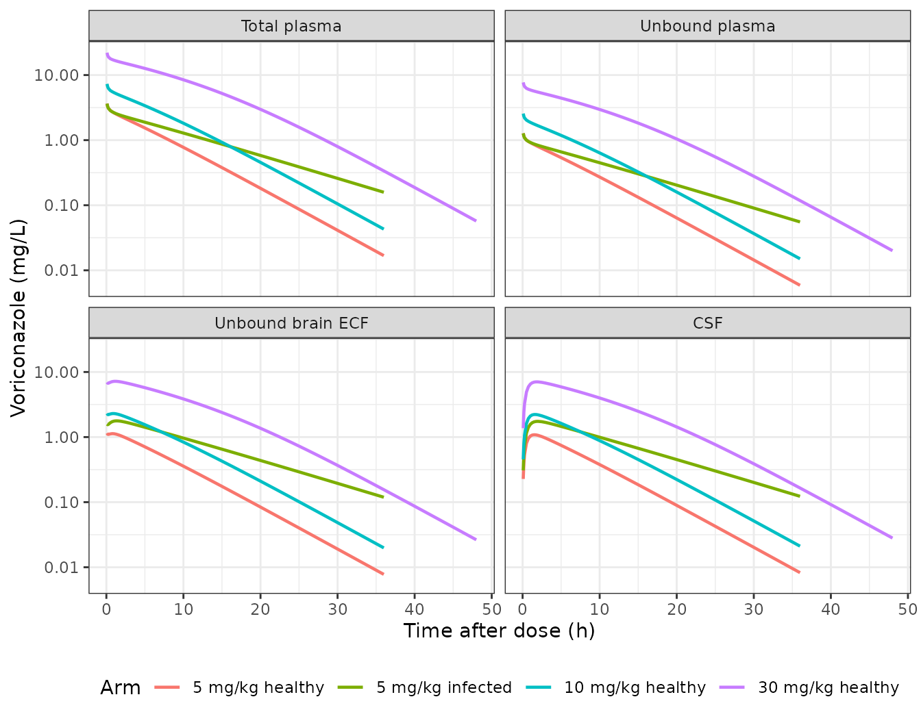
Typical-value profiles after a single intravenous bolus (compare with the observed profiles of Supplementary Figure S1).
The brain extracellular fluid equilibrates with unbound plasma within minutes: Qout / V3 is about 1500 per hour. It then sits above unbound plasma by the ratio Qin / Qout: 1.28 in healthy rats and 2.09 in infected rats. The CSF follows the brain extracellular fluid more slowly, through Q4 / V4 (about 2.5 per hour). Infection raises Km, which slows elimination, and lowers Qout, which traps more drug in the brain.
Figure 3: prediction-corrected VPC medians
Figure 3 of the paper is a prediction-corrected VPC on the natural-log scale. Its solid line is the median of the simulations. This is clear from the CSF panel, where the line ends at about -3.4 at 48 h while the observations sit near -6.5. The maintainers read the line off the published figure at the times below, for the healthy and infected brain (5 mg/kg) and for the CSF (30 mg/kg). The plasma panel pools three dose levels after prediction correction, so it is not compared here. Prediction correction pulls each bin towards the typical prediction, so the read-off median is compared with the typical-value simulation.
fig3 <- tibble::tribble(
  ~panel,            ~arm,               ~time, ~ln_paper,
  "Healthy brain",   "5 mg/kg healthy",  0.5,   0.00,
  "Healthy brain",   "5 mg/kg healthy",  1.5,   0.00,
  "Healthy brain",   "5 mg/kg healthy",  4,     -0.30,
  "Healthy brain",   "5 mg/kg healthy",  6,     -0.58,
  "Healthy brain",   "5 mg/kg healthy",  8,     -0.85,
  "Healthy brain",   "5 mg/kg healthy",  11.5,  -1.33,
  "Infected brain",  "5 mg/kg infected", 1,     0.32,
  "Infected brain",  "5 mg/kg infected", 2,     0.38,
  "Infected brain",  "5 mg/kg infected", 4,     0.25,
  "Infected brain",  "5 mg/kg infected", 6,     0.07,
  "Infected brain",  "5 mg/kg infected", 8,     -0.10,
  "Infected brain",  "5 mg/kg infected", 12,    -0.40,
  "CSF",             "30 mg/kg healthy", 1,     1.80,
  "CSF",             "30 mg/kg healthy", 10,    1.30,
  "CSF",             "30 mg/kg healthy", 48,    -3.40
)

fig3_cmp <- fig3 |>
  rowwise() |>
  mutate(conc_model = {
    d <- bolus_typ[bolus_typ$arm == arm, ]
    y <- if (panel == "CSF") d$Cbrain_csf else d$Cbrain_ecf
    stats::approx(d$time, y, xout = time)$y
  }) |>
  ungroup() |>
  mutate(ln_model = log(conc_model), diff = ln_model - ln_paper)

fig3_cmp |>
  mutate(across(c(ln_model, diff), \(x) round(x, 2))) |>
  select(Panel = panel, `Time (h)` = time, `Figure 3 median (ln mg/L)` = ln_paper,
         `Typical value (ln mg/L)` = ln_model, `Difference (ln units)` = diff) |>
knitr::kable(caption = "Figure 3 simulated medians read off the figure versus this implementation's typical value.")| Panel | Time (h) | Figure 3 median (ln mg/L) | Typical value (ln mg/L) | Difference (ln units) |
|---|---|---|---|---|
| Healthy brain | 0.5 | 0.00 | 0.11 | 0.11 |
| Healthy brain | 1.5 | 0.00 | 0.08 | 0.08 |
| Healthy brain | 4.0 | -0.30 | -0.21 | 0.09 |
| Healthy brain | 6.0 | -0.58 | -0.48 | 0.10 |
| Healthy brain | 8.0 | -0.85 | -0.75 | 0.10 |
| Healthy brain | 11.5 | -1.33 | -1.24 | 0.09 |
| Infected brain | 1.0 | 0.32 | 0.57 | 0.25 |
| Infected brain | 2.0 | 0.38 | 0.55 | 0.17 |
| Infected brain | 4.0 | 0.25 | 0.42 | 0.17 |
| Infected brain | 6.0 | 0.07 | 0.27 | 0.20 |
| Infected brain | 8.0 | -0.10 | 0.12 | 0.22 |
| Infected brain | 12.0 | -0.40 | -0.19 | 0.21 |
| CSF | 1.0 | 1.80 | 1.87 | 0.07 |
| CSF | 10.0 | 1.30 | 1.38 | 0.08 |
| CSF | 48.0 | -3.40 | -3.57 | -0.17 |
# Deterministic (typical-value) solve, so the only error is the read-off of
# the published figure (about 0.05 ln units) and the prediction correction.
# Measured: median difference 0.10, largest 0.25 (infected brain at 1 h).
# Swapping Qin and Qout lowers the healthy-brain and CSF curves by about
# 0.5 ln units, which the median bound rejects.
stopifnot(
  nrow(fig3_cmp) == nrow(fig3),
  !anyNA(fig3_cmp$diff),
  abs(median(fig3_cmp$diff)) < 0.2,
  max(abs(fig3_cmp$diff)) < 0.4
)
The healthy-brain and CSF medians agree within 0.17 ln units (about 15%). The infected-brain median sits about 0.2 ln units (20%) above the figure throughout, a constant offset, so the shape of the curve matches.
vpc_dat <- long_endpoints(bolus_sim) |>
  filter(
    (arm == "5 mg/kg healthy" & matrix == "Unbound brain ECF" & time >= 0.25 & time <= 12) |
      (arm == "5 mg/kg infected" & matrix == "Unbound brain ECF" & time >= 0.25 & time <= 12) |
      (arm == "30 mg/kg healthy" & matrix == "CSF" & time >= 0.25 & time <= 48)
  ) |>
  mutate(panel = case_when(
    matrix == "CSF" ~ "CSF",
    arm == "5 mg/kg healthy" ~ "Healthy brain",
    TRUE ~ "Infected brain"
  )) |>
  group_by(panel, time) |>
  summarise(p10 = quantile(log(conc), 0.1), p50 = median(log(conc)),
            p90 = quantile(log(conc), 0.9), .groups = "drop")

ggplot(vpc_dat, aes(time, p50)) +
  geom_ribbon(aes(ymin = p10, ymax = p90), fill = "#1F6F7A", alpha = 0.25) +
  geom_line(colour = "#1F6F7A") +
  geom_point(data = fig3, aes(time, ln_paper), colour = "black") +
  facet_wrap(~panel, scales = "free") +
  labs(x = "Time after dose (h)", y = "ln voriconazole (mg/L)") +
  theme_bw()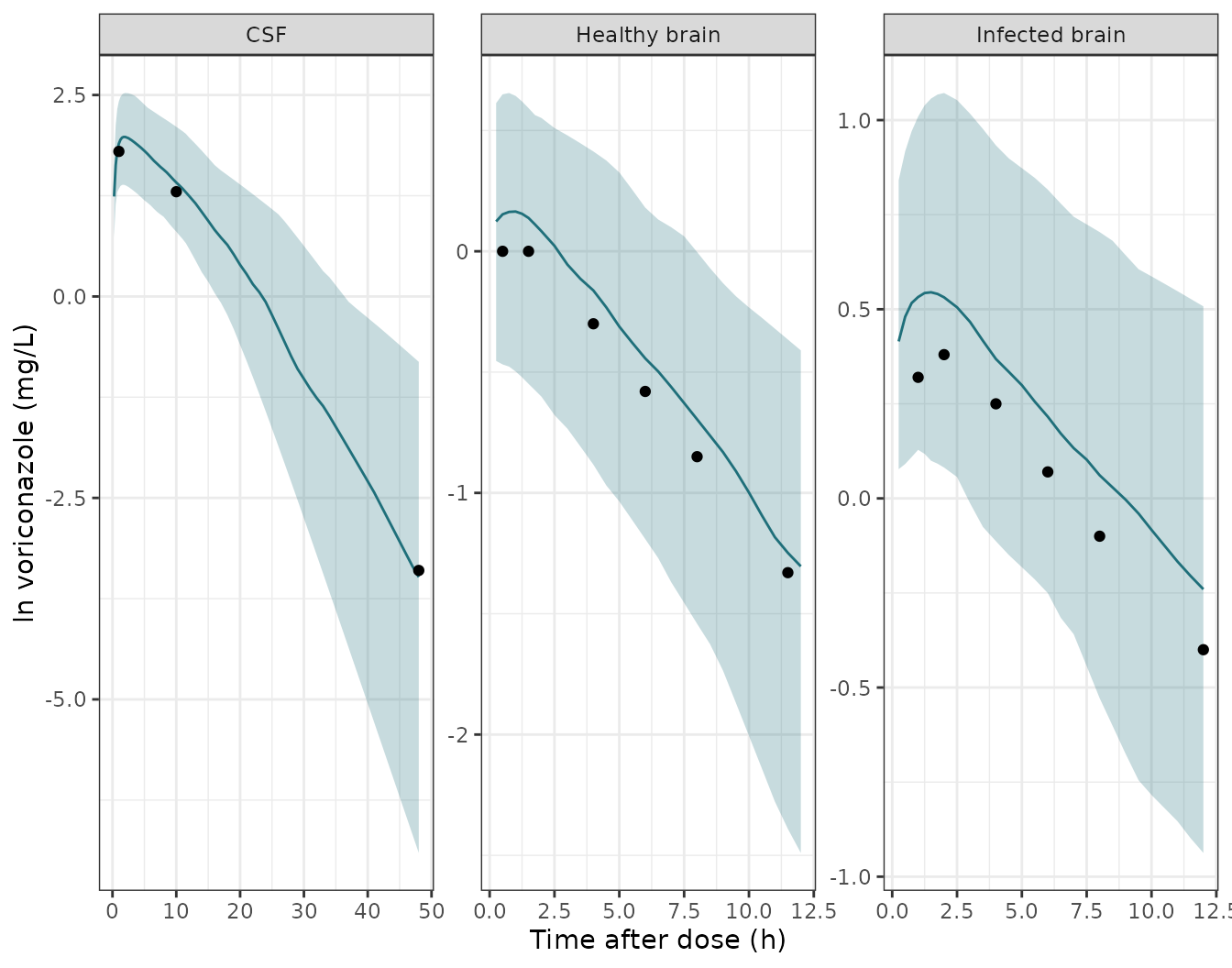
Simulated 10th, 50th and 90th percentiles (100 rats per arm), the percentiles of the pcVPC in Figure 3, on a natural-log axis as in the paper. Points are the medians read off Figure 3.
Mass balance: brain-to-plasma exposure ratio
Drug leaves the brain extracellular fluid and the CSF only by returning to plasma. Integrating Equations 6 and 7 to infinity therefore gives, for every rat, AUC(brain ECF) / AUC(unbound plasma) = Qin / Qout exactly. PKNCA’s AUC0-inf on the simulated profiles has to reproduce each rat’s own Qin / Qout. The remaining difference is purely numerical: trapezoidal error plus the extrapolation past the last sample (36 h, or 48 h at 30 mg/kg).
# The ODE solve undershoots zero by about atol far down the tail; floor it
# and drop the numerically-zero tail after the peak so the log-down
# trapezoid and the half-life fit never see integrator noise.
nca_input <- function(d, conc_col) {
  d |>
    filter(!is.na(.data[[conc_col]])) |>
    select(id, time, arm, conc = all_of(conc_col)) |>
    group_by(id) |>
    filter(time <= time[which.max(conc)] | conc >= 1e-6 * max(conc)) |>
    ungroup() |>
    mutate(conc = pmax(conc, 0))
}
dose_df <- bolus_ev |>
  filter(evid == 1) |>
  select(id, time, amt, arm)
dose_obj <- PKNCA::PKNCAdose(dose_df, amt ~ time | arm + id, route = "intravascular")

run_nca <- function(conc_col, intervals) {
  conc_obj <- PKNCA::PKNCAconc(nca_input(bolus_sim, conc_col), conc ~ time | arm + id)
  res <- PKNCA::pk.nca(PKNCA::PKNCAdata(conc_obj, dose_obj, intervals = intervals))
  as.data.frame(res$result)
}

inf_int <- data.frame(start = 0, end = Inf, aucinf.obs = TRUE)
auc_u <- run_nca("Cu", inf_int)
auc_b <- run_nca("Cbrain_ecf", inf_int)

ratio_chk <- auc_u |>
  filter(PPTESTCD == "aucinf.obs") |>
  select(arm, id, auc_u = PPORRES) |>
  inner_join(auc_b |> filter(PPTESTCD == "aucinf.obs") |>
               select(id, auc_b = PPORRES), by = "id") |>
  inner_join(bolus_sim |> distinct(id, clin, clef), by = "id") |>
  mutate(ratio = auc_b / auc_u, expected = clin / clef,
         pct_diff = 100 * (ratio - expected) / expected)

ratio_chk |>
  group_by(arm) |>
  summarise(`Median AUC ratio` = signif(median(ratio), 3),
            `Median Qin / Qout` = signif(median(expected), 3),
            `Max abs % diff` = signif(max(abs(pct_diff)), 2), .groups = "drop") |>
  rename(Arm = arm) |>
knitr::kable(caption = "Unbound brain-ECF to unbound-plasma AUC0-inf ratio versus each rat's Qin / Qout.")| Arm | Median AUC ratio | Median Qin / Qout | Max abs % diff |
|---|---|---|---|
| 5 mg/kg healthy | 1.33 | 1.34 | 1.20 |
| 5 mg/kg infected | 2.02 | 2.03 | 0.74 |
| 10 mg/kg healthy | 1.30 | 1.31 | 0.87 |
| 30 mg/kg healthy | 1.29 | 1.29 | 0.66 |
Supplementary Table S3: post hoc AUC0-t
Supplementary Table S3 lists AUC0-t of unbound plasma, unbound brain and CSF from the authors’ post hoc predictions, one row per source study. The paper does not give each study’s AUC0-t window. Here 0-12 h is used for the 5 and 10 mg/kg arms (the microdialysis collection period) and 0-48 h for the 30 mg/kg arm (the last CSF sample). Each matrix is a separate PKNCA run.
interval_for <- function(arm_lvl) {
  tend <- if (arm_lvl == "30 mg/kg healthy") 48 else 12
  data.frame(arm = arm_lvl, start = 0, end = tend, auclast = TRUE)
}
s3_int <- dplyr::bind_rows(lapply(levels(arms$arm), interval_for))

s3_sim <- dplyr::bind_rows(
  run_nca("Cu", s3_int) |> mutate(matrix = "Unbound plasma"),
  run_nca("Cbrain_ecf", s3_int) |> mutate(matrix = "Unbound brain"),
  run_nca("Cbrain_csf", s3_int) |> mutate(matrix = "CSF")
) |>
  filter(PPTESTCD == "auclast") |>
  mutate(group = paste(arm, "-", matrix)) |>
  select(group, PPTESTCD, PPORRES)

s3_ref <- tibble::tribble(
  ~group,                                ~auclast,
  "5 mg/kg healthy - Unbound plasma",    7.31,
  "5 mg/kg healthy - Unbound brain",     6.05,
  "5 mg/kg infected - Unbound plasma",   7.42,
  "5 mg/kg infected - Unbound brain",    10.99,
  "10 mg/kg healthy - Unbound plasma",   18.78,
  "30 mg/kg healthy - Unbound plasma",   121.26,
  "30 mg/kg healthy - CSF",              21.36
)

s3_tbl <- ncaComparisonTable(
  s3_sim |> filter(group %in% s3_ref$group),
  s3_ref,
  by = "group",
  units = c(auclast = "mg*h/L")
)
knitr::kable(s3_tbl, caption = "AUC0-t: Supplementary Table S3 popPK-model column (Reference) versus the median of 100 simulated rats per arm.")| NCA parameter | group | Reference | Simulated | % diff |
|---|---|---|---|---|
| AUClast (mg*h/L) | 5 mg/kg healthy - Unbound plasma | 7.31 | 6.16 | -15.7% |
| AUClast (mg*h/L) | 5 mg/kg healthy - Unbound brain | 6.05 | 8.3 | +37.2%* |
| AUClast (mg*h/L) | 5 mg/kg infected - Unbound plasma | 7.42 | 7.62 | +2.7% |
| AUClast (mg*h/L) | 5 mg/kg infected - Unbound brain | 11 | 15.1 | +37.0%* |
| AUClast (mg*h/L) | 10 mg/kg healthy - Unbound plasma | 18.8 | 13.4 | -28.8%* |
| AUClast (mg*h/L) | 30 mg/kg healthy - Unbound plasma | 121 | 72.4 | -40.3%* |
| AUClast (mg*h/L) | 30 mg/kg healthy - CSF | 21.4 | 96.7 | +352.8%* |
- differs from reference by more than ±20%.
The unbound-plasma AUCs at 5 mg/kg agree within about 16%. The study-level post hoc values do not follow from the printed parameters for the brain and CSF, and the paper’s own table shows the same inconsistency:
- Brain-to-plasma ratio. Table S3 gives an unbound brain-to-plasma AUC ratio of 0.83 for healthy rats (6.05 / 7.31) and 1.48 for infected rats. The Discussion quotes 0.82 and 1.50. By the mass balance shown above, the printed Table 1 parameters fix the typical ratio at Qin / Qout: 0.81 / 0.634 = 1.28 healthy and 0.81 / 0.388 = 2.09 infected. A healthy ratio below 1 would need Qin < Qout, i.e. the two values swapped. That reading contradicts the Figure 3 medians, which the printed values match (see above).
- CSF. Table S3 gives a CSF AUC0-48 of 21.36 against an unbound-plasma AUC of 121.26. In the model, drug leaves the CSF only by returning to the brain extracellular fluid. Its AUC must therefore approach the brain AUC, which is above the plasma AUC. No parameter set of this structure gives a CSF exposure one sixth of plasma. Figure 3 again matches the printed parameters.
- 10 and 30 mg/kg plasma. These are under-predicted by about 30% and 40%. The Lelievre rats are Sprague-Dawley and heavier than the reference, and Table S3 for this study is a single naive-pooled profile. The maintainers did not find a weight or window that reconciles them, and no parameter was changed.
Probability of target attainment (Figure 4)
The paper scaled the human voriconazole regimens to rats by basal metabolic rate (Supplementary Equations S1-S2, Table S1). The standard regimen of 6 mg/kg q12h on day 1 then 4 mg/kg q12h becomes 22 then 15 mg/kg q12h in rats. The half-dose regimen (3 then 2 mg/kg in humans) becomes 11 then 7.5 mg/kg. The target was fAUC/MIC > 25. The paper does not state the AUC window or the infusion duration. Here fAUC is the unbound AUC over the second day (24-48 h) after intravenous boluses, and the CSF is taken as unbound (Equation 3 gives an unbound CSF fraction of 0.994 for rats). There are 200 virtual rats per regimen and group.
n_pta <- 200L
regimens <- tibble::tribble(
  ~regimen,                 ~load_mgkg, ~maint_mgkg,
  "Standard (6 / 4 mg/kg)", 22,         15,
  "Half dose (3 / 2 mg/kg)", 11,        7.5
)
pta_design <- tidyr::expand_grid(regimens, DIS_INFECT_ACTIVE = c(0L, 1L)) |>
  mutate(group = ifelse(DIS_INFECT_ACTIVE == 1L, "Infected", "Healthy"))

pta_events <- function(i) {
  r <- pta_design[i, ]
  ev <- rxode2::et(amt = r$load_mgkg * rat_wt, ii = 12, addl = 1, cmt = "central") |>
    rxode2::et(amt = r$maint_mgkg * rat_wt, time = 24, ii = 12, addl = 1, cmt = "central") |>
    rxode2::et(seq(24, 48, by = 0.1), cmt = "central") |>
    as.data.frame()
  ev$dvid <- ifelse(ev$evid == 0, 1L, NA_integer_)
  tidyr::expand_grid(id = seq_len(n_pta) + (i - 1L) * n_pta, ev) |>
    mutate(WT = rat_wt, DIS_INFECT_ACTIVE = r$DIS_INFECT_ACTIVE,
           regimen = r$regimen, group = r$group)
}
pta_ev <- dplyr::bind_rows(lapply(seq_len(nrow(pta_design)), pta_events)) |>
  arrange(id, time, desc(evid))

rxode2::rxSetSeed(2024)
pta_sim <- rxode2::rxSolve(mod, pta_ev, keep = c("regimen", "group"),
                           useLinCmt = FALSE) |>
  as.data.frame()

trap <- function(t, y) sum(diff(t) * (head(y, -1) + tail(y, -1)) / 2)
fauc <- pta_sim |>
  filter(time >= 24, time <= 48) |>
  group_by(regimen, group, id) |>
  summarise(Plasma = trap(time, Cu), ISF = trap(time, Cbrain_ecf),
            CSF = trap(time, Cbrain_csf), .groups = "drop") |>
  pivot_longer(c(Plasma, ISF, CSF), names_to = "matrix", values_to = "fauc") |>
  mutate(matrix = factor(matrix, levels = c("Plasma", "ISF", "CSF")))

mics <- 2^seq(-9, 9) # 0.002 to 512 mg/L
pta <- fauc |>
  tidyr::expand_grid(mic = mics) |>
  group_by(regimen, group, matrix, mic) |>
  summarise(pta = 100 * mean(fauc / mic > 25), .groups = "drop")
# Figure 4, read by the maintainers. Both regimens' panels in the published
# figure are identical, so one set of values is listed.
fig4 <- tibble::tribble(
  ~group,     ~matrix,  ~mic, ~paper,
  "Healthy",  "Plasma", 2,    98,
  "Healthy",  "Plasma", 4,    31,
  "Healthy",  "Plasma", 8,    0,
  "Healthy",  "ISF",    2,    88,
  "Healthy",  "ISF",    4,    37,
  "Healthy",  "ISF",    8,    2,
  "Healthy",  "CSF",    2,    88,
  "Healthy",  "CSF",    4,    38,
  "Healthy",  "CSF",    8,    3,
  "Infected", "Plasma", 2,    99,
  "Infected", "Plasma", 4,    55,
  "Infected", "Plasma", 8,    0,
  "Infected", "ISF",    4,    81,
  "Infected", "ISF",    8,    23,
  "Infected", "CSF",    4,    85,
  "Infected", "CSF",    8,    29
)

pta |>
  filter(regimen == "Standard (6 / 4 mg/kg)") |>
  mutate(matrix = as.character(matrix)) |>
  inner_join(fig4, by = c("group", "matrix", "mic")) |>
  select(Group = group, Matrix = matrix, `MIC (mg/L)` = mic,
         `Figure 4 PTA (%)` = paper, `Simulated PTA (%)` = pta) |>
knitr::kable(caption = "PTA for fAUC/MIC > 25, standard regimen: Figure 4 versus this implementation (200 rats per group).")| Group | Matrix | MIC (mg/L) | Figure 4 PTA (%) | Simulated PTA (%) |
|---|---|---|---|---|
| Healthy | Plasma | 2 | 98 | 91.0 |
| Healthy | Plasma | 4 | 31 | 31.5 |
| Healthy | Plasma | 8 | 0 | 2.0 |
| Healthy | ISF | 2 | 88 | 93.5 |
| Healthy | ISF | 4 | 37 | 54.5 |
| Healthy | ISF | 8 | 2 | 13.5 |
| Healthy | CSF | 2 | 88 | 93.5 |
| Healthy | CSF | 4 | 38 | 54.5 |
| Healthy | CSF | 8 | 3 | 14.0 |
| Infected | Plasma | 2 | 99 | 99.5 |
| Infected | Plasma | 4 | 55 | 71.5 |
| Infected | Plasma | 8 | 0 | 6.0 |
| Infected | ISF | 4 | 81 | 98.0 |
| Infected | ISF | 8 | 23 | 69.5 |
| Infected | CSF | 4 | 85 | 98.0 |
| Infected | CSF | 8 | 29 | 69.5 |
ggplot(pta, aes(mic, pta, colour = matrix)) +
  geom_line() +
  geom_point(size = 1) +
  geom_hline(yintercept = 90, linetype = "dashed") +
  facet_grid(regimen ~ group) +
  scale_x_log10() +
  labs(x = "MIC (mg/L)", y = "PTA (%)", colour = "Matrix") +
  theme_bw() +
  theme(legend.position = "bottom")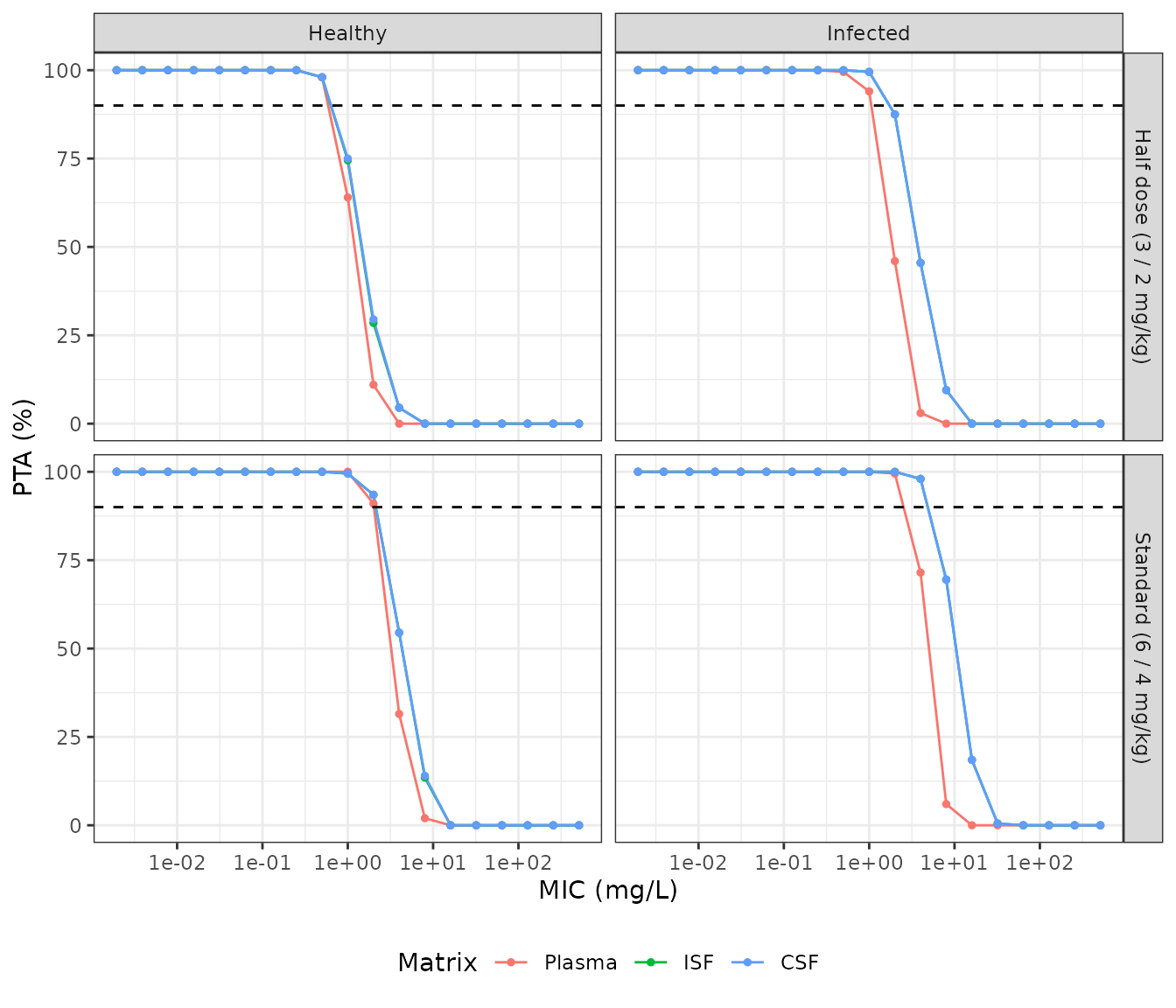
PTA across the EUCAST MIC range for each regimen, group and matrix (replicates Figure 4 of Staudt 2023). The dashed line marks 90% PTA.
The paper’s conclusions are checked below. Every matrix and both groups reach more than 90% PTA at the most prevalent C. neoformans MICs (0.06 and 0.125 mg/L), and on to 1 mg/L, under the standard regimen. The bounds are far from the simulated values, so the cohort draw cannot flip them.
std <- pta |> filter(regimen == "Standard (6 / 4 mg/kg)")
stopifnot(
  all(std$pta[std$mic <= 1] > 90),
  all(pta$pta[pta$mic <= 0.125] > 90),
  all(std$pta[std$mic >= 64] < 10)
)
Under the standard regimen, the simulated PTA falls through 90% between 2 and 8 mg/L, as in Figure 4. Because the brain-to-plasma ratio is above 1 here (see “Supplementary Table S3” above), the ISF and CSF curves sit to the right of the plasma curve in both groups. In the published figure they overlap the plasma curve in healthy rats. The half-dose regimen shifts the curves left by about a factor of two to three. The published Figure 4 shows identical curves for the two regimens, which is not possible for a model with Michaelis-Menten elimination.
Assumptions and deviations
-
Km is an amount. Equation 4 writes the elimination
as
Vmax * A1 / (Km + A1)with the unbound central amount A1, while Table 1, the abstract and the Results label Km in mg/L. The model follows the printed equation, so Km is in mg. Two things support this reading. The authors scale Km allometrically with the same 0.75 exponent as Vmax, which fits an amount rather than a concentration. And the paper’s unit labels are unreliable elsewhere: Q1 is printed in L, Qin and Qout in 1/h in the abstract, and Qout in mg/L in the Results. With V1 = 1.15 L the concentration reading would be equivalent to a Km of 5.5 mg. Across the 5-30 mg/kg doses the two readings change the unbound-plasma AUC by less than 10%, so neither Figure 3 nor Table S3 can tell them apart. - Infected parameters. Equations 8 and 9 as printed are not usable (they give Km = 0 for a healthy rat, and Equation 9 repeats the infected theta). The Results say Km and Qout “were calculated separately for the infected group” and give the infected values. The model uses separate typical values for each group. The more precise text values (Km 4.76 and 8.135; Qout 0.634 and 0.388) are used in place of Table 1’s rounded 8.13, 0.63 and 0.38. The bootstrap medians in Table 1 for Km,infected (0.68) and Qout,infected (0.35) suggest the estimated thetas were fractional effects. Either way the infected typical values are those printed.
- Q4 connects brain and CSF. The parameter list after Equation 7 calls Q4 the clearance “from the central compartment to CSF”. Equations 6-7 and Figure 1 connect the CSF to the brain compartment, and the model follows them.
- Reference body weight. The median weight in Equation 1 is not reported. The model uses 0.35 kg, the rat mass the same paper uses for its dose scaling. All simulations here use 0.35 kg rats, so the parameters equal Table 1 and the reference choice has no effect on them.
- Unbound fraction. The model divides unbound plasma by 0.35 to give total plasma (Results). Methods state 66% protein binding (unbound fraction 0.34), and the Discussion uses 0.34. The model uses 0.35 as the Results state for the fit.
-
CSF concentrations. Total CSF concentrations were
fitted directly to A4 / V4. The model returns that quantity as
Cbrain_csf. - Residual and IIV scales. The log-additive errors (0.107, 0.074, 0.450) are encoded as SDs on the log scale. IIV percentages are taken as log-normal CVs: omega^2 = log(CV^2 + 1).
- Microdialysate collection intervals. The authors fitted microdialysate data as the integral over each collection interval. The model returns the instantaneous unbound concentration; to fit interval data, average the prediction over each interval.
- Inconsistent derived results. The Table S3 brain and CSF post hoc AUCs, the Discussion’s penetration ratios and the overlap of the plasma and ISF PTA curves in healthy rats (Figure 4) all disagree with the printed parameters. The printed parameters are consistent with Equations 4-7 and reproduce the Figure 3 medians. The model follows the printed parameters and no value was tuned.
- PTA set-up. The AUC window and administration mode for Figure 4 are not stated. The second dosing day after intravenous boluses is an assumption. The paper’s correction of the rat Kp,uu,CSF to humans is not reproduced.