Letrozole in rat plasma and brain (Arora 2021)

Model and source

• Citation: Arora P, Gudelsky G, Desai PB. Gender-based differences in brain and plasma pharmacokinetics of letrozole in sprague-dawley rats: Application of physiologically-based pharmacokinetic modeling to gain quantitative insights. PLoS ONE. 2021;16(4):e0248579. doi:10.1371/journal.pone.0248579. PMCID PMC8018653. Drug-specific PBPK inputs are Table 1 (with footnotes a and b giving the per-kg clearance and per-gram PSB they were derived from) and Eq 3 (Crone-Renkin PSB). PBPK-predicted versus observed NCA metrics are Table 4 (single dose) and Table 5 (steady state); observed NCA is Tables 2 and 3; individual observed concentrations are Supporting Information Tables S1 and S2 (figshare doi:10.6084/m9.figshare.14184959.v1).
• Description: Preclinical (rat). PBPK-derived reduced model (Simcyp Animal Simulator V17) for letrozole in plasma and brain extracellular fluid (ECF) of male and female Sprague-Dawley rats after single and once-daily 4 mg/kg extravascular doses. The source paper built a bottom-up whole-body PBPK model with the Simcyp multi-compartment brain model (brain blood, brain mass, CSF); the rat organ volumes, blood flows, tissue compositions and the Rodgers-Rowland tissue partition coefficients are Simcyp library values that are not printed, so the whole-body structure is not reproduced. What the paper does print (Table 1) is a complete systemic card – first-order absorption rate and fraction absorbed, the in vivo oral clearance entered as the clearance input, and the predicted steady-state volume of distribution – plus the brain permeability-surface area product across the blood-brain barrier and the unbound fractions in plasma and brain. This file encodes a one-compartment first-order-absorption plasma model with V = Vss and CL/F = CLpo, and a brain-mass compartment exchanging unbound drug with plasma across the blood-brain barrier at the printed PSB; brain ECF concentration is the unbound brain concentration fu,brain times total brain concentration, exactly as the paper derives it. The CSF compartment (printed PSC and PSE, but unprinted CSF volume, bulk flow and CSF sink flow) and the brain blood compartment (unprinted volume and cerebral blood flow) are omitted. Clearance and absorption rate differ by sex (females clear letrozole about 3.7-fold more slowly); volume and brain parameters are shared. With zero fitted parameters, the reduction reproduces all 18 PBPK-predicted plasma and brain ECF exposure metrics of Tables 4 and 5 within 12% (14 within 5%). Typical-value model: the paper reports no interindividual or residual variability, so no etas are declared and all residual error terms are fixed at zero.
• Article: https://doi.org/10.1371/journal.pone.0248579
• Supporting information (individual concentrations): https://doi.org/10.6084/m9.figshare.14184959.v1

Arora 2021 measured letrozole in plasma and in brain extracellular fluid (ECF, by striatal microdialysis) of male and female Sprague-Dawley rats after a single 4 mg/kg intraperitoneal dose and at steady state (once daily for 5 days in males, 11 days in females). Female rats cleared letrozole several-fold more slowly than males, so plasma and brain exposure were much higher in females. The authors then built a bottom-up whole-body PBPK model in the Simcyp Animal Simulator V17, with the Simcyp multi-compartment brain model (brain blood, brain mass and CSF), and compared its predictions with the observed exposures (Tables 4 and 5).

Why a reduced model

The Simcyp rat physiology (organ volumes, blood flows, tissue composition) and the Rodgers-Rowland tissue partition coefficients it computes are Simcyp library values that are not printed in the paper, so the whole-body structure cannot be rebuilt. The paper does print the complete drug card (Table 1):

• first-order absorption rate Ka and fraction absorbed Fa,
• the in vivo oral clearance CLpo that was entered as the clearance input,
• the predicted steady-state volume of distribution Vss, and
• for the brain, the blood-brain barrier permeability-surface area product PSB and the unbound fractions in plasma and brain.

This file therefore encodes a one-compartment first-order-absorption plasma model with V = Vss and CL/F = CLpo, plus a brain compartment that exchanges unbound drug with plasma across the blood-brain barrier at PSB. Brain ECF is fu,brain times the total brain concentration, which is how the paper itself converts simulated brain tissue to ECF (Figure 4 and 5 captions). No parameter was fitted. The comparison section below shows that the reduction reproduces all 18 PBPK-predicted exposure metrics in Tables 4 and 5 within 12%.

Population

The observed study used 10 female (201-225 g) and 10 male (301-325 g) age-matched (7-9 weeks) jugular-vein-cannulated Sprague-Dawley rats (Methods, “Animals”); 3-6 rats per group contributed data (Tables 2 and 3). The PBPK model was not fitted to these rats. Its absorption and clearance came from an earlier oral-gavage study in rats (Liu 2000, reference 16 of the paper), its volume from the Rodgers-Rowland prediction, and its brain parameters from an in situ brain perfusion Kin and an in vivo fu,brain measurement. Doses are per kg, and clearance and volume scale linearly with body weight, so plasma and brain ECF concentrations do not depend on the weight chosen for the simulation.

The same information is available programmatically via readModelDb("Arora_2021_letrozole_rat")()$population.

Source trace

Equation / parameter	Value	Source location
lka (males)	log(0.29) 1/h	Table 1, Ka 0.29 (males)
e_sexf_ka	log(0.49) - log(0.29)	Table 1, Ka 0.49 (females)
lfdepot	log(0.99)	Table 1, Fa 0.99
lcl (males, per kg)	log(0.77 x 0.06 / 0.25) = log(0.1848) L/h/kg	Table 1, CLpo 0.77 mL/min; footnote a (0.185 L/h/kg at 250 g)
e_sexf_cl	log(0.21) - log(0.77)	Table 1, CLpo 0.21 mL/min (females); footnote a (0.051 L/h/kg)
lvc (per kg)	log(3.29) L/kg	Table 1, Vss 3.29 L/kg (Rodgers-Rowland, Kp scalar 1)
lps_bbb	log(0.84 x 0.06) L/h	Table 1, PSB 0.84 mL/min; Eq 3 (Crone-Renkin); footnote b
lvbrain	log(0.0018) L	Table 1 footnote b, 1800 mg brain weight
fu_plasma	0.4	Table 1, fraction unbound in plasma
fu_brain	0.58	Table 1, fraction unbound in brain; Methods (0.58 +/- 0.19)
kel = CLpo x F / V	–	Reduction: systemic CL = F x CLpo, so AUC = Dose / CLpo
d/dt(brain) = PSB (fu_p Cp - fu_brain Cbrain)	–	Figure 1 (passive PSB at the BBB)
Cecf = fu_brain x Cbrain	–	Methods “PBPK modeling and simulation”; Figure 4 and 5 captions
Residual error	fixed 0	Not reported

PSC (0.42 mL/min) and PSE (80 mL/min) in Table 1 belong to the CSF compartment, which is omitted (see Assumptions).

Simulation

The model has no between-subject variability, so each arm is a single typical rat. Weight is set to 0.25 kg, the body weight Table 1 footnote a assumes.

mod <- readModelDb("Arora_2021_letrozole_rat")
wt <- 0.25
dose_mg <- 4 * wt

arms <- tibble::tribble(
  ~arm,                  ~SEXF, ~n_doses, ~regimen, ~sex,
  "Male, single dose",   0,     1,        "single", "male",
  "Female, single dose", 1,     1,        "single", "female",
  "Male, day 5",         0,     5,        "ss",     "male",
  "Female, day 11",      1,     11,       "ss",     "female"
) |>
  mutate(id = seq_len(n()), t_last = (n_doses - 1) * 24)

make_events <- function(a) {
  dose_times <- (seq_len(a$n_doses) - 1) * 24
  obs_end <- a$t_last + ifelse(a$regimen == "single", 72, 24)
  obs_times <- sort(unique(c(seq(0, obs_end, by = 0.5),
                             seq(a$t_last, a$t_last + 24, by = 0.05))))
  bind_rows(
    tibble(time = dose_times, amt = dose_mg, evid = 1L, cmt = "depot",
           dvid = NA_integer_),
    # Observe on the ODE state `central` with dvid = 1: the model has two
    # endpoints (Cc, Cecf), and rxSolve returns both columns on every row.
    tibble(time = obs_times, amt = 0, evid = 0L, cmt = "central", dvid = 1L)
  ) |>
    mutate(id = a$id, SEXF = a$SEXF, WT = wt)
}
events <- bind_rows(lapply(split(arms, arms$id), make_events)) |>
  arrange(id, time, desc(evid))

sim <- rxode2::rxSolve(mod, events = events, returnType = "data.frame",
                       atol = 1e-10, rtol = 1e-10) |>
  left_join(arms |> select(id, arm, regimen, sex, t_last), by = "id") |>
  mutate(tad = time - t_last)
#> Warning: multi-subject simulation without without 'omega'

Mass balance

Elimination is only from the central compartment, so the plasma AUC to infinity after a single dose must equal F x Dose / CL_systemic = Dose / CLpo. A long single-dose solve checks it for both sexes.

mb_events <- bind_rows(
  tibble(id = 1:2, time = 0, amt = dose_mg, evid = 1L, cmt = "depot",
         dvid = NA_integer_),
  tidyr::expand_grid(id = 1:2, time = c(seq(0, 48, by = 0.02),
                                        seq(48.5, 3000, by = 0.5))) |>
    mutate(amt = 0, evid = 0L, cmt = "central", dvid = 1L)
) |>
  mutate(SEXF = id - 1, WT = wt) |>
  arrange(id, time, desc(evid))
mb <- rxode2::rxSolve(mod, events = mb_events, returnType = "data.frame",
                      atol = 1e-12, rtol = 1e-12)
#> Warning: multi-subject simulation without without 'omega'
auc_trap <- mb |>
  group_by(id) |>
  summarise(auc = sum(diff(time) * (head(Cc, -1) + tail(Cc, -1)) / 2)) |>
  mutate(
    clpo_L_h = c(0.77, 0.21) * 0.06,          # Table 1 CLpo at 250 g
    expected = dose_mg / clpo_L_h * 1000,     # ng*h/mL
    pct_diff = 100 * (auc / expected - 1)
  )
knitr::kable(auc_trap, digits = 3,
             caption = "Plasma AUC0-inf vs Dose / CLpo (typical 250 g rat).")

Plasma AUC0-inf vs Dose / CLpo (typical 250 g rat).

id	auc	clpo_L_h	expected	pct_diff
1	21645.13	0.046	21645.02	0
2	79365.25	0.013	79365.08	0

stopifnot(all(abs(auc_trap$pct_diff) < 0.5))

Replicate published figures

The observed individual concentrations are Supporting Information Tables S1 (single dose) and S2 (steady state). Brain ECF values there are already corrected for the 7.2% in vitro probe recovery. The steady-state time 0 is the pre-dose trough on the last dosing day.

obs_list <- list(
  data.frame(
    regimen = "single", sex = "male", matrix = "plasma",
    time = c(
      0, 0, 0, 0, 1, 1, 1, 1, 2, 2, 2, 2, 4, 4, 4, 4, 6, 6, 6, 6, 8, 8, 8,
      8, 12, 12, 12, 12, 14, 14, 14, 14, 20, 20, 20, 20, 24, 24, 24, 24, 36,
      36, 36, 36, 48, 48, 48, 48, 72, 72, 72
    ),
    conc = c(
      0, 0, 0, 0, 1044.393, 876.391, 591.211, 1199.197, 1063.636, 925.246,
      510.069, 1228.875, 984.805, 1012.029, 559.271, 1414.03, 1091.724,
      1023.698, 553.350, 1520.244, 1055.773, 1001.363, 617.079, 1002.802,
      929.884, 870.730, 501.609, 758.094, 844.281, 888.179, 474.035,
      811.867, 587.719, 730.852, 389.702, 447.428, 478.275, 554.283,
      365.418, 335.743, 218.882, 312.336, 256.352, 123.051, 59.396, 130.541,
      229.735, 31.813, 9.323, 36.685, 3.422
    )
  ),
  data.frame(
    regimen = "single", sex = "female", matrix = "plasma",
    time = c(
      0, 0, 0, 0, 1, 1, 1, 1, 2, 2, 2, 2, 4, 4, 4, 4, 6, 6, 6, 6, 8, 8, 8,
      8, 12, 12, 12, 12, 14, 14, 14, 14, 20, 20, 20, 20, 24, 24, 24, 24, 36,
      36, 36, 36, 48, 48, 48, 48, 72, 72, 72, 72
    ),
    conc = c(
      0, 0, 0, 0, 720.571, 623.175, 1052.091, 480.031, 856.193, 838.972,
      1148.68, 591.951, 1051.717, 1043.124, 1290.945, 814.589, 1183.064,
      1079.904, 1355.867, 1100.971, 1075.217, 1084.742, 1319.881, 834.645,
      1003.936, 1015.505, 1239.973, 768.096, 1096.256, 1136.607, 1345.730,
      813.860, 1040.732, 984.403, 1231.618, 891.091, 931.895, 955.263,
      1164.917, 681.496, 820.211, 769.045, 943.573, 738.413, 579.921,
      563.092, 726.495, 454.573, 364.006, 328.232, 454.143, 303.522
    )
  ),
  data.frame(
    regimen = "single", sex = "male", matrix = "ecf",
    time = c(
      0, 0, 0, 1, 1, 1, 2, 2, 2, 4, 4, 4, 6, 6, 6, 8, 8, 8, 12, 12, 12
    ),
    conc = c(
      0, 0, 0, 210.327, 52.067, 101.302, 244.195, 200.338, 181.835, 305.393,
      179.345, 227.999, 293.519, 131.230, 212.045, 340.403, 135.092,
      202.727, 323.880, 102.487, 167.753
    )
  ),
  data.frame(
    regimen = "single", sex = "female", matrix = "ecf",
    time = c(
      0, 0, 0, 0, 1, 1, 1, 1, 2, 2, 2, 2, 4, 4, 4, 4, 6, 6, 6, 8, 8, 8, 12,
      12, 12
    ),
    conc = c(
      0, 0, 0, 0, 85.949, 187.391, 313.810, 157.184, 216.717, 461.903,
      837.136, 322.733, 369.765, 610.928, 969.232, 410.723, 392.790,
      431.902, 490.683, 450.539, 501.163, 537.898, 459.484, 429.908, 600.978
    )
  ),
  data.frame(
    regimen = "ss", sex = "male", matrix = "plasma",
    time = c(
      0, 0, 0, 0, 0, 0, 1, 1, 1, 1, 1, 1, 2, 2, 2, 2, 2, 2, 4, 4, 4, 4, 4,
      4, 6, 6, 6, 6, 6, 6, 8, 8, 8, 8, 8, 8, 12, 12, 12, 12, 12, 12, 24, 24,
      24, 24, 24, 24
    ),
    conc = c(
      708.371, 914.583, 306.278, 249.293, 626.040, 430.870, 1380.867,
      2091.997, 840.374, 905.873, 1335.739, 1202.517, 1546.278, 2302.436,
      890.533, 784.141, 1215.889, 1336.560, 1717.487, 2138.971, 911.896,
      712.757, 1107.499, 1292.113, 1940.414, 2169.134, 1018.459, 655.777,
      1067.159, 1276.933, 2010.057, 2035.74, 839.752, 549.749, 958.455,
      1134.681, 1702.384, 1827.786, 557.692, 431.903, 808.769, 960.670,
      1056.352, 1182.492, 262.335, 189.933, 460.088, 584.849
    )
  ),
  data.frame(
    regimen = "ss", sex = "female", matrix = "plasma",
    time = c(
      0, 0, 0, 0, 1, 1, 1, 1, 2, 2, 2, 2, 4, 4, 4, 4, 6, 6, 6, 6, 8, 8, 8,
      8, 12, 12, 12, 12, 24, 24, 24, 24
    ),
    conc = c(
      3939.162, 3106.762, 3409.916, 3114.453, 4171.520, 3948.940, 4129.197,
      3903.636, 4393.729, 4036.905, 3952.161, 3702.467, 4616.463, 3909.576,
      4286.518, 3778.609, 4255.196, 4134.814, 4119.688, 3771.741, 5657.767,
      5464.587, 4128.687, 3833.352, 5016.707, 5421.316, 4165.648, 3633.862,
      4176.895, 4381.714, 3995.076, 3434.456
    )
  ),
  data.frame(
    regimen = "ss", sex = "male", matrix = "ecf",
    time = c(
      0, 0, 0, 0, 0, 1, 1, 1, 1, 1, 1, 2, 2, 2, 2, 2, 2, 4, 4, 4, 4, 4, 4,
      6, 6, 6, 6, 6, 6, 8, 8, 8, 8, 8, 8, 12, 12, 12, 12, 12, 12
    ),
    conc = c(
      309.891, 323.454, 454.744, 269.963, 218.834, 376.201, 401.986,
      496.912, 486.570, 357.648, 222.341, 425.834, 442.384, 640.105,
      412.280, 404.770, 304.824, 419.456, 432.772, 689.791, 356.564,
      400.349, 264.563, 412.894, 421.338, 708.967, 337.511, 371.685,
      271.920, 399.034, 403.237, 752.531, 289.348, 363.384, 259.305,
      320.956, 327.492, 583.700, 266.138, 330.116, 216.533
    )
  ),
  data.frame(
    regimen = "ss", sex = "female", matrix = "ecf",
    time = c(
      0, 0, 0, 1, 1, 1, 1, 1, 1, 2, 2, 2, 2, 2, 2, 4, 4, 4, 4, 4, 4, 6, 6,
      6, 6, 6, 6, 8, 8, 8, 8, 8, 8, 12, 12, 12, 12, 12, 12
    ),
    conc = c(
      2247.026, 976.794, 1531.236, 2186.254, 1935.792, 2191.154, 2567.958,
      1165.727, 1711.756, 2704.617, 1604.792, 2211.754, 2453.834, 1234.575,
      1710.061, 2745.388, 1512.549, 2017.898, 2664.161, 1371.678, 1621.921,
      3117.949, 1719.762, 2053.278, 2865.700, 1376.413, 2161.965, 2227.750,
      1875.563, 2146.324, 2595.646, 1324.437, 1914.079, 2258.556, 1910.011,
      2178.404, 2642.540, 1394.720, 2228.501
    )
  )
)
obs <- do.call(rbind, obs_list)
obs_summary <- obs |>
  group_by(regimen, sex, matrix, time) |>
  summarise(mean = mean(conc), sd = sd(conc), n = n(), .groups = "drop")

# Replicates Figure 4 of Arora 2021: single dose, plasma (A, B) and brain ECF
# (C, D), male and female.
pred_long <- sim |>
  select(arm, regimen, sex, tad, Cc, Cecf) |>
  pivot_longer(c(Cc, Cecf), names_to = "matrix", values_to = "conc") |>
  mutate(matrix = ifelse(matrix == "Cc", "plasma", "ecf"))

plot_arm <- function(reg, xmax_plasma) {
  p <- pred_long |>
    filter(regimen == reg, tad >= 0,
           (matrix == "plasma" & tad <= xmax_plasma) |
             (matrix == "ecf" & tad <= 12))
  o <- obs_summary |> filter(regimen == reg)
  ggplot() +
    geom_line(data = p, aes(tad, conc), linetype = "dashed") +
    geom_pointrange(data = o,
                    aes(time, mean, ymin = pmax(mean - sd, 0), ymax = mean + sd),
                    size = 0.2) +
    facet_wrap(~ factor(matrix, c("plasma", "ecf"),
                        c("Plasma", "Brain ECF")) + sex,
               scales = "free") +
    labs(x = "Time after dose (h)", y = "Letrozole (ng/mL)")
}
plot_arm("single", 72) +
  labs(title = "Single 4 mg/kg dose",
       caption = paste("Replicates Figure 4 of Arora 2021. Dashed: model;",
                       "points: observed mean +/- SD (Table S1)."))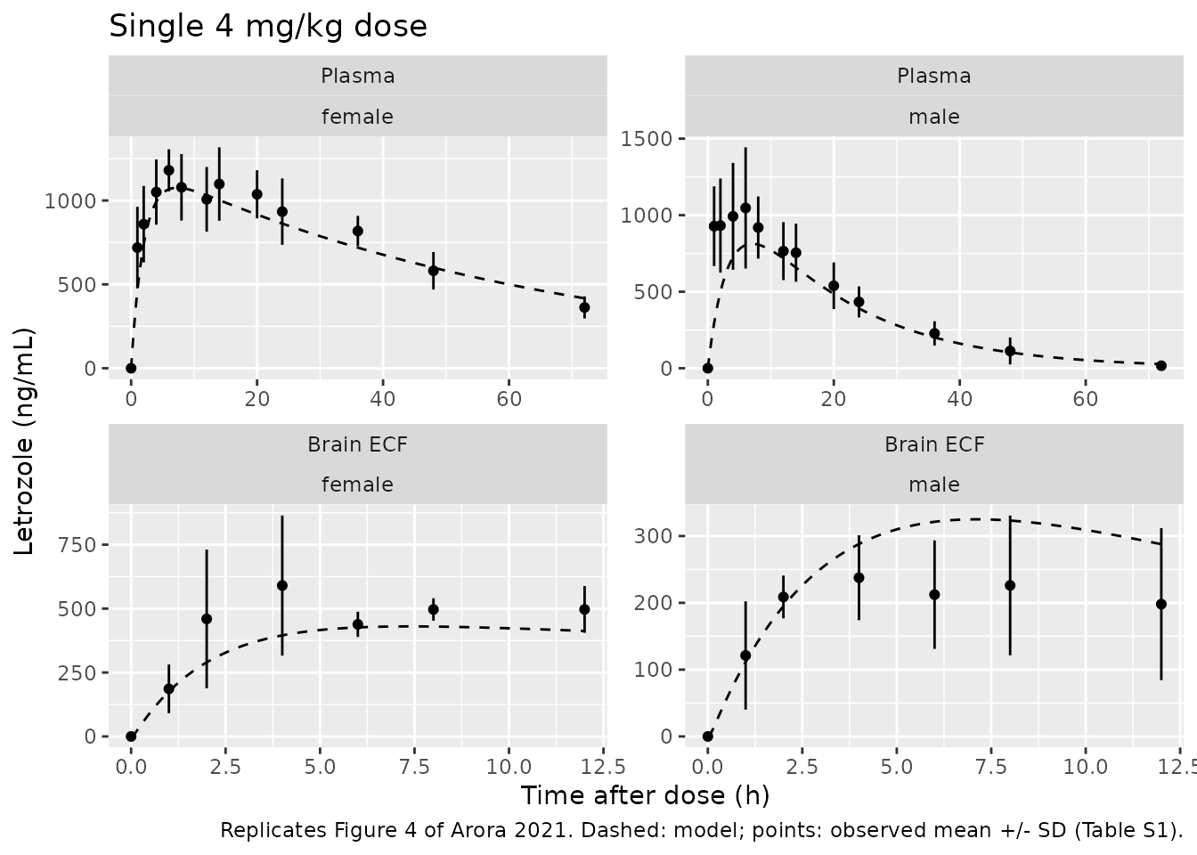

# Replicates Figure 5 of Arora 2021: last dose at steady state (day 5 males,
# day 11 females).
plot_arm("ss", 24) +
  labs(title = "Steady state, 4 mg/kg once daily",
       caption = paste("Replicates Figure 5 of Arora 2021. Dashed: model;",
                       "points: observed mean +/- SD (Table S2)."))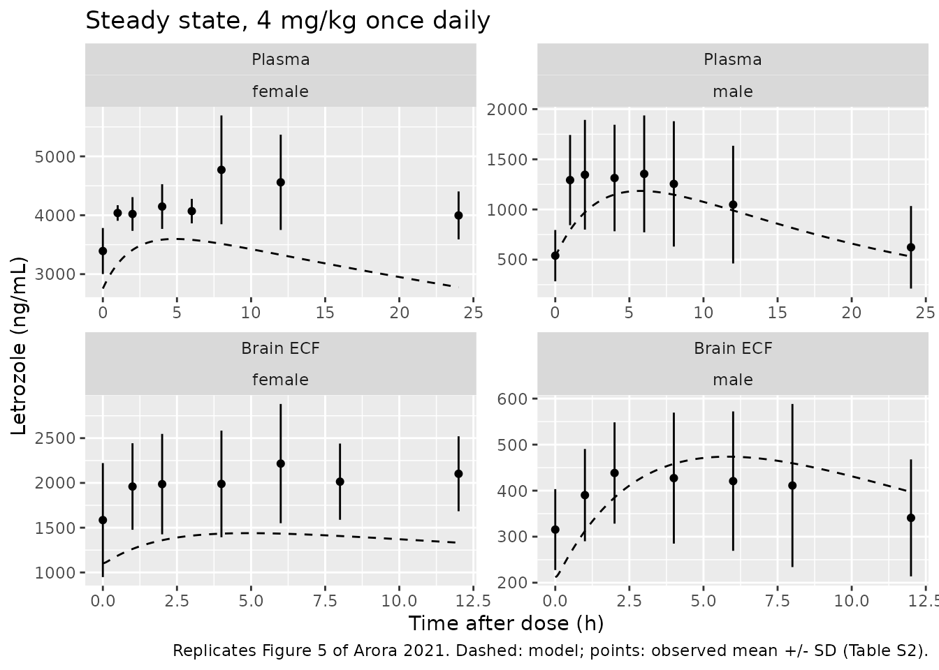

PKNCA validation

Plasma and brain ECF are analysed as separate groups over the windows the paper used: plasma 0-72 h and brain ECF 0-12 h after a single dose; plasma 0-24 h and brain ECF 0-12 h after the last steady-state dose.

nca_conc <- sim |>
  select(arm, regimen, t_last, time, Cc, Cecf) |>
  pivot_longer(c(Cc, Cecf), names_to = "analyte", values_to = "conc") |>
  mutate(matrix = ifelse(analyte == "Cc", "Plasma", "Brain ECF")) |>
  filter(!is.na(conc)) |>
  mutate(group = paste(arm, matrix, sep = " | "),
         id = as.integer(factor(group))) |>
  select(id, group, arm, matrix, regimen, t_last, time, conc)

nca_groups <- nca_conc |> distinct(id, group, arm)
nca_dose <- events |>
  filter(evid == 1) |>
  select(sim_id = id, time, amt) |>
  left_join(arms |> select(sim_id = id, arm), by = "sim_id") |>
  inner_join(nca_groups, by = "arm", relationship = "many-to-many") |>
  select(id, group, time, amt)

intervals <- nca_conc |>
  distinct(id, group, matrix, regimen, t_last) |>
  mutate(
    start = t_last,
    end = t_last + case_when(
      matrix == "Brain ECF" ~ 12,
      regimen == "single" ~ 72,
      TRUE ~ 24
    ),
    cmax = TRUE,
    auclast = TRUE,
    half.life = regimen == "single" & matrix == "Plasma"
  ) |>
  select(id, group, start, end, cmax, auclast, half.life)

conc_obj <- PKNCA::PKNCAconc(nca_conc, conc ~ time | group + id,
                             concu = "ng/mL", timeu = "h")
dose_obj <- PKNCA::PKNCAdose(nca_dose, amt ~ time | group + id, doseu = "mg")
nca_res <- PKNCA::pk.nca(PKNCA::PKNCAdata(conc_obj, dose_obj,
                                          intervals = as.data.frame(intervals)))

Comparison against the paper’s PBPK predictions

The reduction’s job is to reproduce what the Simcyp model predicted, so the reference is the Predicted column of Tables 4 (single dose) and 5 (steady state). auclast is AUC0-72 (single-dose plasma), AUC0-24 (steady-state plasma) or AUC0-12 (brain ECF).

published <- tibble::tribble(
  ~group,                             ~cmax, ~auclast, ~half.life,
  "Male, single dose | Plasma",        790,   21050,   13.34,
  "Female, single dose | Plasma",     1080,   51870,   43.77,
  "Male, single dose | Brain ECF",     310,    3120,      NA,
  "Female, single dose | Brain ECF",   470,    4640,      NA,
  "Male, day 5 | Plasma",             1190,   21640,      NA,
  "Female, day 11 | Plasma",          3650,   79310,      NA,
  "Male, day 5 | Brain ECF",           470,    5140,      NA,
  "Female, day 11 | Brain ECF",       1510,   18730,      NA
)

sim_nca <- as.data.frame(nca_res$result) |>
  filter(PPTESTCD %in% c("cmax", "auclast", "half.life")) |>
  select(group, PPTESTCD, PPORRES)

cmp <- nlmixr2lib::ncaComparisonTable(
  simulated = sim_nca,
  reference = published,
  by = "group",
  units = c(cmax = "ng/mL", auclast = "ng*h/mL", half.life = "h"),
  tolerance_pct = 20
)
knitr::kable(cmp, caption = paste(
  "Reduced model vs the Simcyp PBPK predictions of Arora 2021 Tables 4-5.",
  "* differs from the reference by more than 20%."
))

Reduced model vs the Simcyp PBPK predictions of Arora 2021 Tables 4-5. * differs from the reference by more than 20%.

NCA parameter	group	Reference	Simulated	% diff
Cmax (ng/mL)	Male, single dose | Plasma	790	813	+2.9%
Cmax (ng/mL)	Female, single dose | Plasma	1080	1080	-0.4%
Cmax (ng/mL)	Male, single dose | Brain ECF	310	325	+4.8%
Cmax (ng/mL)	Female, single dose | Brain ECF	470	430	-8.5%
Cmax (ng/mL)	Male, day 5 | Plasma	1190	1180	-0.5%
Cmax (ng/mL)	Female, day 11 | Plasma	3650	3600	-1.4%
Cmax (ng/mL)	Male, day 5 | Brain ECF	470	474	+0.8%
Cmax (ng/mL)	Female, day 11 | Brain ECF	1510	1440	-4.7%
AUClast (ng*h/mL)	Male, single dose | Plasma	21000	21200	+0.5%
AUClast (ng*h/mL)	Female, single dose | Plasma	51900	51800	-0.1%
AUClast (ng*h/mL)	Male, single dose | Brain ECF	3120	3200	+2.7%
AUClast (ng*h/mL)	Female, single dose | Brain ECF	4640	4410	-5.0%
AUClast (ng*h/mL)	Male, day 5 | Plasma	21600	21600	-0.1%
AUClast (ng*h/mL)	Female, day 11 | Plasma	79300	77900	-1.8%
AUClast (ng*h/mL)	Male, day 5 | Brain ECF	5140	5070	-1.5%
AUClast (ng*h/mL)	Female, day 11 | Brain ECF	18700	16500	-11.8%
t½ (h)	Male, single dose | Plasma	13.3	12.6	-5.6%
t½ (h)	Female, single dose | Plasma	43.8	46	+5.1%

pct <- suppressWarnings(as.numeric(gsub("[^0-9.+-]", "", cmp[["% diff"]])))
pct <- pct[!is.na(pct)]
stopifnot(
  # The model is deterministic (no random effects), so these are fixed
  # numbers: a mis-transcribed clearance, volume, dose or unit moves every
  # row by tens of percent.
  length(pct) == 18,
  all(abs(pct) < 15),
  abs(median(pct)) < 5
)

Every metric lands within 15% of the Simcyp prediction, and 14 of 18 within 5%. The largest gaps are in the female brain ECF (single-dose Cmax about 9% low, steady-state AUC0-12 about 12% low). In the reduced model the ECF/plasma peak ratio is 0.40 in both sexes, the plasma unbound fraction that a purely passive blood-brain barrier gives at equilibrium. The Simcyp predictions give 0.39-0.40 in males but 0.41-0.44 in females. The difference must come from the omitted brain-blood and CSF compartments or other unprinted Simcyp internals, and the printed parameters cannot resolve it. The simulated single-dose plasma half-lives come from PKNCA’s terminal fit over 0-72 h and sit about 6% below (males) and 5% above (females) the Simcyp values, consistent with ln2 x Vss / (F x CLpo) = 12.5 h and 45.7 h.

Comparison against the observed data

For context, the observed exposures of Tables 2 and 3 are listed next to the same simulated values. These rats were not used to build the model; the paper reports the predicted/observed ratios as 0.66-1.45 (Tables 4 and 5).

observed <- tibble::tribble(
  ~group,                             ~cmax, ~auclast,
  "Male, single dose | Plasma",       1060,   24860,
  "Female, single dose | Plasma",     1200,   54390,
  "Male, single dose | Brain ECF",     260,    2410,
  "Female, single dose | Brain ECF",   660,    5750,
  "Male, day 5 | Plasma",             1490,   24800,
  "Female, day 11 | Plasma",          4830,  102970,
  "Male, day 5 | Brain ECF",           490,    4820,
  "Female, day 11 | Brain ECF",       2290,   23990
)
cmp_obs <- nlmixr2lib::ncaComparisonTable(
  simulated = sim_nca,
  reference = observed,
  by = "group",
  params = c("cmax", "auclast"),
  units = c(cmax = "ng/mL", auclast = "ng*h/mL"),
  tolerance_pct = 30
)
knitr::kable(cmp_obs, caption = paste(
  "Reduced model vs observed means of Arora 2021 Tables 2-3.",
  "* differs from the observed mean by more than 30%."
))

Reduced model vs observed means of Arora 2021 Tables 2-3. * differs from the observed mean by more than 30%.

NCA parameter	group	Reference	Simulated	% diff
Cmax (ng/mL)	Male, single dose | Plasma	1060	813	-23.3%
Cmax (ng/mL)	Female, single dose | Plasma	1200	1080	-10.4%
Cmax (ng/mL)	Male, single dose | Brain ECF	260	325	+25.0%
Cmax (ng/mL)	Female, single dose | Brain ECF	660	430	-34.8%*
Cmax (ng/mL)	Male, day 5 | Plasma	1490	1180	-20.5%
Cmax (ng/mL)	Female, day 11 | Plasma	4830	3600	-25.5%
Cmax (ng/mL)	Male, day 5 | Brain ECF	490	474	-3.3%
Cmax (ng/mL)	Female, day 11 | Brain ECF	2290	1440	-37.2%*
AUClast (ng*h/mL)	Male, single dose | Plasma	24900	21200	-14.9%
AUClast (ng*h/mL)	Female, single dose | Plasma	54400	51800	-4.7%
AUClast (ng*h/mL)	Male, single dose | Brain ECF	2410	3200	+32.9%*
AUClast (ng*h/mL)	Female, single dose | Brain ECF	5750	4410	-23.3%
AUClast (ng*h/mL)	Male, day 5 | Plasma	24800	21600	-12.9%
AUClast (ng*h/mL)	Female, day 11 | Plasma	103000	77900	-24.4%
AUClast (ng*h/mL)	Male, day 5 | Brain ECF	4820	5070	+5.1%
AUClast (ng*h/mL)	Female, day 11 | Brain ECF	24000	16500	-31.2%*

The female steady-state exposures are under-predicted by about 24-37%, as they are by the Simcyp model itself (predicted/observed 0.66-0.78, Table 5). The male single-dose brain ECF is over-predicted by 25-33%, again in line with the Simcyp model (predicted/observed 1.19-1.29, Table 4). The paper attributes the extra accumulation in females (observed 4-fold versus a predicted 2.6-fold) to possible saturation of hepatic metabolism, which a linear model cannot represent.

Assumptions and deviations

• Whole-body structure reduced to one compartment. The Simcyp rat organ volumes, blood flows, tissue compositions and Rodgers-Rowland partition coefficients are not printed. The plasma layer uses the printed Vss as the single volume. The reduction is checked against the paper’s own predicted exposures above rather than assumed.
• Bioavailability is Fa. Table 1 prints Fa = 0.99 but not the gut or hepatic first-pass fractions, which Simcyp derives internally. The model takes F = Fa and systemic clearance F x CLpo, which keeps AUC = Dose / CLpo exact (the definition of the entered in vivo oral clearance). A hepatic extraction below 1 would lower the predicted Cmax by a few percent.
• Dosing route. The rats were dosed intraperitoneally, but the paper simulated “extravascular” first-order absorption with the oral-gavage Ka of reference 16. The model follows the simulation (depot with first-order absorption).
• Per-kg scaling. Clearance and volume are scaled linearly by body weight, following Table 1 (Vss in L/kg; CLpo derived from a per-kg clearance at an assumed 250 g). With per-kg doses, concentrations do not depend on weight. The brain parameters are absolute (PSB for an assumed 1.8 g brain) and are not scaled.
• Brain model reduced to a single brain-mass compartment. The Simcyp multi-compartment brain model also has a brain-blood compartment (fed by cerebral blood flow) and a CSF compartment (exchanging via PSC 0.42 mL/min and PSE 80 mL/min, with bulk flow and a CSF sink flow). The brain-blood volume, cerebral blood flow, CSF volume, bulk flow and CSF sink flow are Simcyp library values that are not printed, so those two compartments are omitted, and the printed PSC and PSE are not used. The brain-mass compartment exchanges directly with unbound plasma drug at the printed PSB, with a volume equal to the assumed 1.8 g brain weight. Because this exchange equilibrates within minutes, brain ECF closely tracks fu_plasma x Cc.
• Brain compartment is mass-conserving. Drug taken up by the brain leaves the central compartment. Since Vss already includes the brain, this counts the brain volume twice; the brain holds about 0.15% of the distribution volume, so the effect is negligible.
• Unbound fractions. Table 1 gives fu_plasma = 0.4, while the Table 2 and 3 footnotes and the Methods use 0.38 for the observed unbound plasma concentrations. The model uses the PBPK input, 0.4.
• No variability. The Simcyp simulations used virtual rat populations, but no variance is reported. No etas are declared and the residual-error terms are fixed at zero.
• Brain ECF recovery. The observed brain ECF values in Tables S1 and S2 are already corrected for the 7.2% in vitro probe recovery. The model predicts ECF directly and needs no recovery correction.