Clarithromycin (Abduljalil 2009)
Source:vignettes/articles/Abduljalil_2009_clarithromycin.Rmd
Abduljalil_2009_clarithromycin.RmdModel and source
- Citation: Abduljalil K, Kinzig M, Bulitta J, Horkovics-Kovats S, Sorgel F, Rodamer M, Fuhr U. Modeling the autoinhibition of clarithromycin metabolism during repeated oral administration. Antimicrob Agents Chemother. 2009 Jul;53(7):2892-2901. doi:10.1128/AAC.01193-08. PMID 19414575.
- Article: https://doi.org/10.1128/AAC.01193-08
- The full structural description, parameter source-trace comments,
and population metadata are carried by the model function itself; load
it with
readModelDb("Abduljalil_2009_clarithromycin")to inspect.
Population
Abduljalil et al. (2009) enrolled 12 healthy adult Caucasian volunteers (7 men, 5 women), ages 19-41 years (mean 28, SD 8), weights 45.1-86.1 kg (mean 66.5, SD 11.8), heights 150-186 cm, at a single centre in the Republic of Moldova. Each subject took oral clarithromycin 500 mg every 12 h for 7 doses (4 consecutive days, dose 7 was the morning dose of day 4). Blood was sampled densely (15 timepoints) over 12 h after doses 1, 3, and 7, plus trough samples before doses 5 and 6. Plasma clarithromycin and 14-(R)-hydroxy-clarithromycin were quantified by LC-MS/MS with LLOQ approximately 0.01 ug/mL.
The packaged model carries the same demographic metadata as
readModelDb("Abduljalil_2009_clarithromycin")$meta$population.
Structural model and source trace
The model couples a single-phase Weibull absorption into a one-compartment parent disposition, an effect-compartment-style hypothetical inhibition compartment driving Imax-style modulation of the parent’s apparent clearance, and a parallel one-compartment metabolite disposition. The complete derivation is in Abduljalil 2009 Methods (Model development) and Figure 2.
| Equation / parameter | Value | Source location |
|---|---|---|
Weibull cumulative
WB(Tw) = 1 - exp[-(kw*Tw)^lambda]
|
- | Methods, Model development, paragraph 2 |
Allometric CL_i = CL * (BW/70)^0.75
|
exponent 0.75 (fixed) | Methods, Model development, paragraph 4 |
Allometric V_i = V * (BW/70)^1.00
|
exponent 1.00 (fixed) | Methods, Model development, paragraph 4 |
Inhibition factor
INH = FCLp + (1-FCLp)/(1 + C_inh/IC50)
|
- | Methods, Model development, paragraph 3; Figure 2 |
d/dt(effect) = ki * (Cp - effect) |
- | Figure 2 (effect-compartment formulation) |
Metabolite formation f_m = 1 (all CLp feeds
metabolite) |
- | Discussion, paragraph 4 |
| kw (Weibull absorption rate constant) | 0.56 1/h (95% CI 0.42-0.69) | Table 1 |
| lambda (Weibull shape) | 2.23 (95% CI 1.67-2.77) | Table 1 |
| Vp (apparent parent central volume) | 172 L (95% CI 145-198) | Table 1 |
| CLp (apparent parent basic clearance) | 60 L/h (95% CI 40-80) | Table 1 |
| FCLp (fraction of CLp not subject to inhibition) | 0.10 (95% CI 0.02-0.17) | Table 1 |
| ki (inhibition-compartment exchange rate) | 2.01 1/h (95% CI 0.09-3.93) | Table 1 |
| IC50 (50% inhibition concentration) | 0.77 ug/mL (95% CI 0.23-1.28) | Table 1 |
| CL_met (apparent metabolite clearance) | 50.2 L/h (95% CI 42.3-58.1) | Table 1 |
| V_met (apparent metabolite central volume) | 34 L (95% CI 12-56) | Table 1 |
| BSV CV(kw) = 45.3 % | omega^2 = log(1 + 0.453^2) | Table 1 |
| BSV CV(Vp) = 25.3 % | omega^2 = log(1 + 0.253^2) | Table 1 |
| BSV CV(CLp) = 17.4 % | omega^2 = log(1 + 0.174^2) | Table 1 |
| BSV CV(CL_met) = 27.9 % | omega^2 = log(1 + 0.279^2) | Table 1 |
| Additive residual SD (parent) | 0.12 ug/mL | Table 1 |
| Additive residual SD (metabolite) | 0.01 ug/mL | Table 1 |
Virtual cohort
The original concentration-time data are not publicly available. The figures below use a virtual cohort of 100 subjects whose body weights are drawn from a truncated normal distribution matching the reported summary statistics (mean 66.5 kg, SD 11.8 kg, support 45-90 kg).
set.seed(20260531)

make_cohort <- function(n, dose_mg, id_offset = 0L, tau = 12, ndoses = 7,
                        obs_end = ndoses * tau) {
  ids <- id_offset + seq_len(n)
  wts <- pmin(pmax(rnorm(n, mean = 66.5, sd = 11.8), 45), 90)

  dose_rows <- expand.grid(id = ids, time = seq(0, by = tau, length.out = ndoses)) |>
    dplyr::mutate(evid = 1L, amt = dose_mg, cmt = "depot")

  # One observation cmt is enough; the model computes Cc and Cc_ohcla
  # together at every solve step (and at every evid=0 observation row),
  # so a single Cc-cmt observation grid keeps the output one-row-per-time
  # without sacrificing the metabolite output.
  obs_grid <- sort(unique(c(seq(0, obs_end, by = 0.25), seq(0, 12, by = 0.05))))
  obs_rows <- expand.grid(id = ids, time = obs_grid) |>
    dplyr::mutate(evid = 0L, amt = 0, cmt = "Cc")

  wt_lookup <- tibble::tibble(id = ids, WT = wts, dose_mg = dose_mg)

  dplyr::bind_rows(dose_rows, obs_rows) |>
    dplyr::left_join(wt_lookup, by = "id") |>
    dplyr::arrange(id, time, dplyr::desc(evid))
}

events <- make_cohort(n = 100, dose_mg = 500)
stopifnot(!anyDuplicated(unique(events[, c("id", "time", "evid", "cmt")])))
Simulation
mod <- readModelDb("Abduljalil_2009_clarithromycin")
mod_typical <- rxode2::zeroRe(mod)
#> ℹ parameter labels from comments will be replaced by 'label()'

# Stochastic VPC over 100 subjects, 500 mg b.i.d.
sim_vpc <- rxode2::rxSolve(mod, events = events,
                           keep = c("WT", "dose_mg"),
                           returnType = "data.frame")
#> ℹ parameter labels from comments will be replaced by 'label()'

# Typical-value (no IIV) replications used by the figure overlays.
sim_typ500 <- rxode2::rxSolve(
  mod_typical,
  events = make_cohort(n = 1L, dose_mg = 500),
  keep = c("WT", "dose_mg"),
  returnType = "data.frame"
)
#> ℹ omega/sigma items treated as zero: 'etalka', 'etalvc', 'etalcl', 'etalcl_ohcla'
Figure 1 – first-dose profile (parent vs metabolite)
sim_d1 <- sim_typ500 |>
  dplyr::filter(time <= 12)

tidy_d1 <- sim_d1 |>
  dplyr::transmute(
    time,
    Clarithromycin                  = Cc,
    `14-(R)-hydroxy-clarithromycin` = Cc_ohcla
  ) |>
  tidyr::pivot_longer(-time, names_to = "Analyte", values_to = "Conc")

ggplot(tidy_d1, aes(time, Conc, colour = Analyte)) +
  geom_line(linewidth = 0.8) +
  labs(x = "Time after dose 1 (h)", y = "Plasma concentration (ug/mL)",
       title = "Figure 1 -- first-dose profile (500 mg)",
       caption = "Replicates Figure 1 of Abduljalil 2009 (Weibull absorption typical values).") +
  theme_minimal()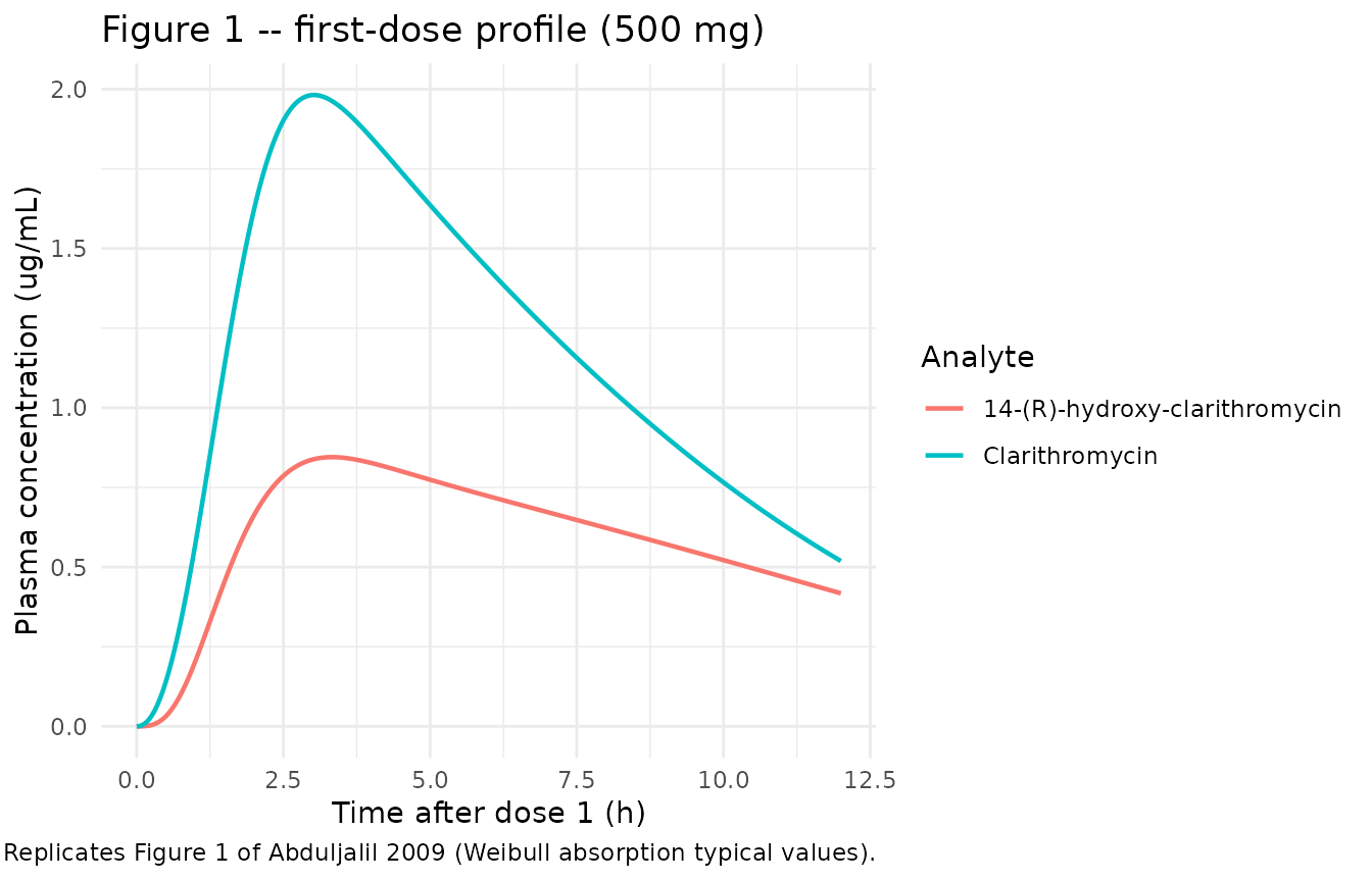
Figure 5 – inhibition compartment and INH(t) at 500 mg b.i.d.
sim_inh <- sim_typ500 |>
  dplyr::select(time, effect, inh)

p_a <- ggplot(sim_inh, aes(time, effect)) +
  geom_line(linewidth = 0.8) +
  labs(x = "Time (h)", y = "Inhibition-compartment\nconcentration (ug/mL)",
       title = "Figure 5A -- inhibition compartment, 500 mg b.i.d.") +
  theme_minimal()

p_b <- ggplot(sim_inh, aes(time, 100 * inh)) +
  geom_line(linewidth = 0.8) +
  geom_hline(yintercept = 10, linetype = "dashed", colour = "grey50") +
  geom_hline(yintercept = 100, linetype = "dotted", colour = "grey50") +
  labs(x = "Time (h)", y = "Overall inhibition parameter INH (%)",
       caption = paste(
         "Replicates Figure 5 of Abduljalil 2009.",
         "INH = 100 % (no inhibition) at C_inh = 0;",
         "asymptote at 10 % (= FCLp, non-inhibitable fraction).")) +
  theme_minimal()

print(p_a)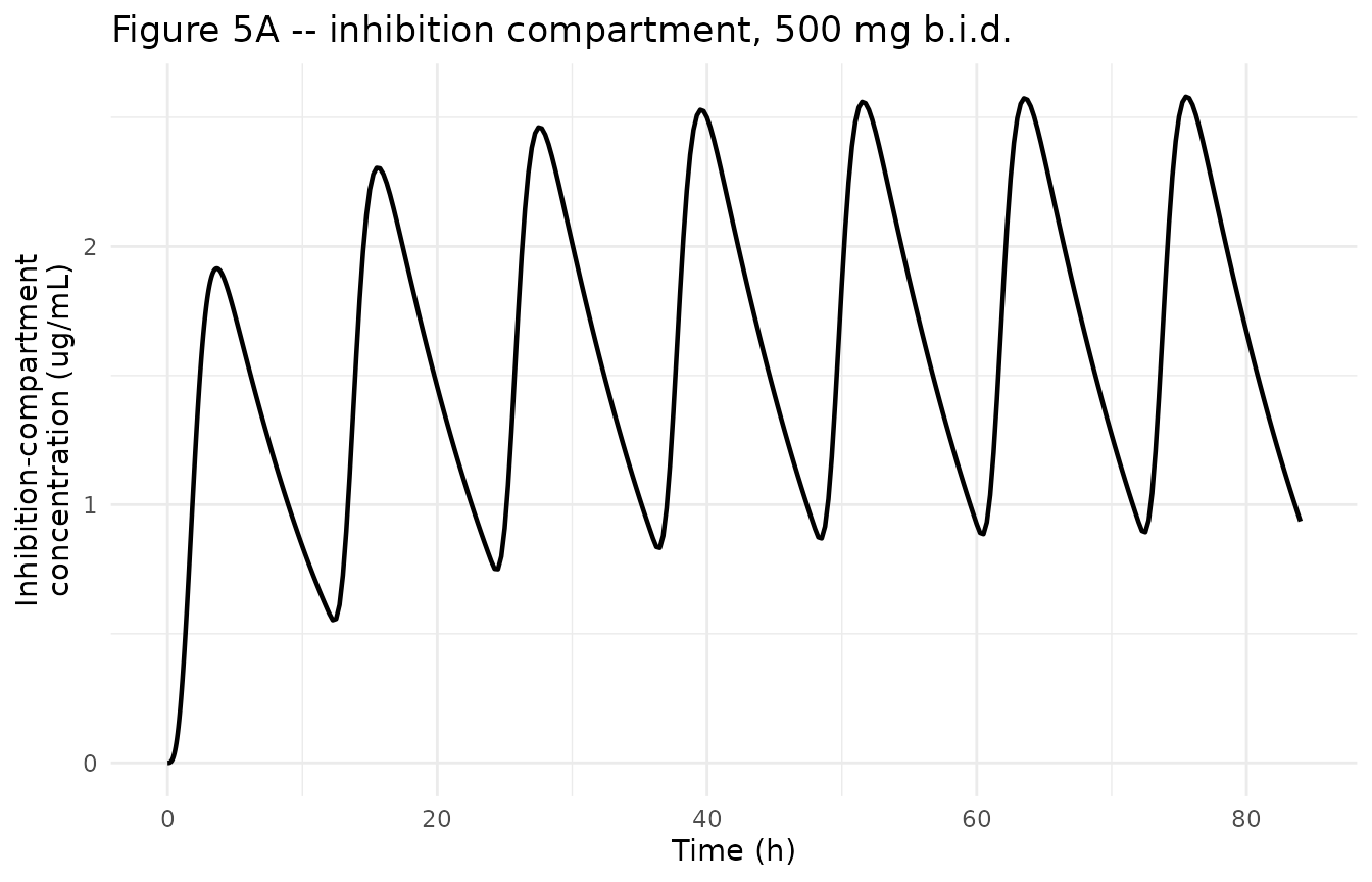
print(p_b)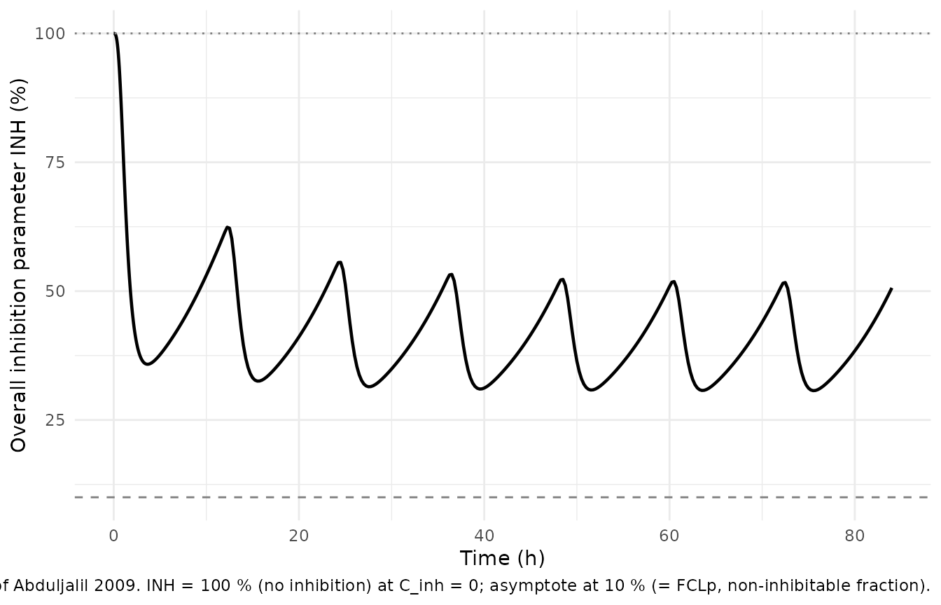
Figure 6 – dose comparison: 250, 500, 750, 1000 mg b.i.d.
dose_levels <- c(250, 500, 750, 1000)
sims_doses <- lapply(seq_along(dose_levels), function(i) {
  d <- dose_levels[i]
  ev <- make_cohort(n = 1L, dose_mg = d, ndoses = 14)
  rxode2::rxSolve(mod_typical, events = ev,
                  keep = c("WT", "dose_mg"),
                  returnType = "data.frame") |>
    dplyr::mutate(dose_label = sprintf("%d mg b.i.d.", d))
})
sim_doses <- dplyr::bind_rows(sims_doses) |>
  dplyr::filter(!is.na(Cc), time <= 168) |>
  dplyr::mutate(
    dose_label = factor(dose_label, levels = sprintf("%d mg b.i.d.", dose_levels))
  )

ggplot(sim_doses, aes(time, Cc, colour = dose_label)) +
  geom_line(linewidth = 0.7) +
  labs(x = "Time (h)", y = "Plasma clarithromycin (ug/mL)",
       colour = "Dose",
       title = "Figure 6 -- typical-value clarithromycin at 250 / 500 / 750 / 1000 mg b.i.d.",
       caption = "Replicates Figure 6 of Abduljalil 2009: time-dependent autoinhibition accumulates more strongly at higher doses.") +
  theme_minimal()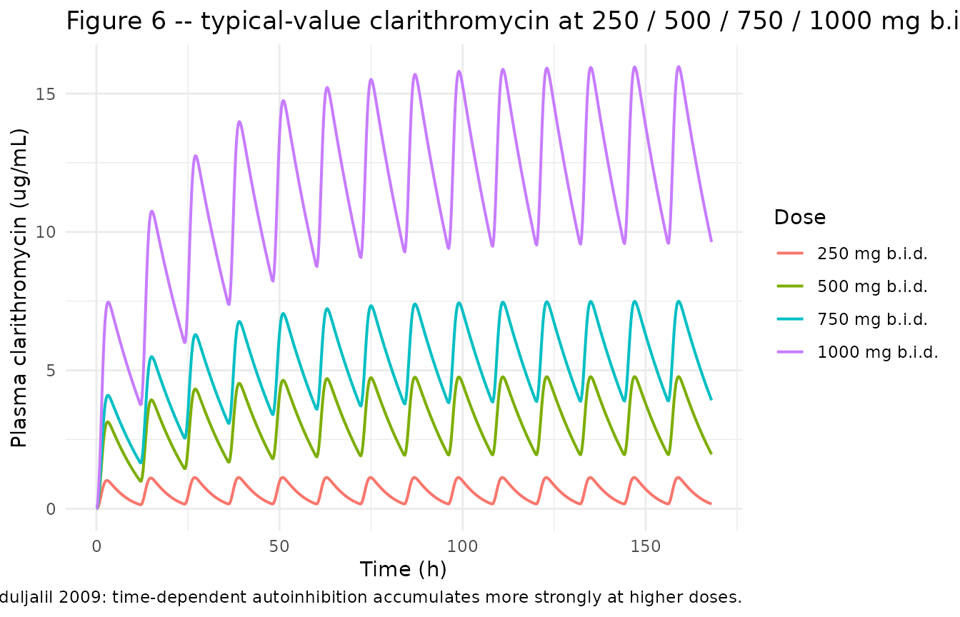
PKNCA validation – Table 2 fAUC comparison
The paper’s Table 2 reports the free-drug AUC over 0-24 h (“initial”) and at steady state for clarithromycin at 250, 500, 750, and 1000 mg b.i.d., assuming free fraction f = 0.30 (Introduction, paragraph 1: “the free fraction of clarithromycin in plasma is about 0.3”). PKNCA computes total AUC; multiplying by 0.30 yields the fAUC values that can be compared with Table 2.
# Long simulation so steady state is reached for fAUC SS comparison.
make_long_cohort <- function(n, dose_mg, tau = 12, ndoses = 30,
                             obs_end = ndoses * tau, id_offset = 0L) {
  ids <- id_offset + seq_len(n)
  dose_rows <- expand.grid(id = ids, time = seq(0, by = tau, length.out = ndoses)) |>
    dplyr::mutate(evid = 1L, amt = dose_mg, cmt = "depot")
  obs_grid <- seq(0, obs_end, by = 0.5)
  obs_rows  <- expand.grid(id = ids, time = obs_grid) |>
    dplyr::mutate(evid = 0L, amt = 0, cmt = "Cc")
  dplyr::bind_rows(dose_rows, obs_rows) |>
    dplyr::mutate(WT = 70, dose_mg = dose_mg) |>
    dplyr::arrange(id, time, dplyr::desc(evid))
}

dose_levels <- c(250, 500, 750, 1000)
auc_sims <- lapply(seq_along(dose_levels), function(i) {
  d <- dose_levels[i]
  ev <- make_long_cohort(n = 1L, dose_mg = d, id_offset = (i - 1L) * 10L)
  rxode2::rxSolve(mod_typical, events = ev,
                  keep = c("WT", "dose_mg"),
                  returnType = "data.frame") |>
    dplyr::filter(!is.na(Cc)) |>
    dplyr::mutate(treatment = sprintf("%d mg b.i.d.", d), dose_mg = d)
})
#> ℹ omega/sigma items treated as zero: 'etalka', 'etalvc', 'etalcl', 'etalcl_ohcla'
#> ℹ omega/sigma items treated as zero: 'etalka', 'etalvc', 'etalcl', 'etalcl_ohcla'
#> ℹ omega/sigma items treated as zero: 'etalka', 'etalvc', 'etalcl', 'etalcl_ohcla'
#> ℹ omega/sigma items treated as zero: 'etalka', 'etalvc', 'etalcl', 'etalcl_ohcla'
sim_auc <- dplyr::bind_rows(auc_sims)

# Compute AUC by trapezoidal rule directly (PKNCA's multi-dose accumulation
# pattern requires more boilerplate than buys here).
fauc_initial <- sim_auc |>
  dplyr::filter(time >= 0, time <= 24) |>
  dplyr::group_by(treatment) |>
  dplyr::arrange(time, .by_group = TRUE) |>
  dplyr::summarise(
    AUC_total = sum(diff(time) * (Cc[-1] + Cc[-dplyr::n()]) / 2),
    .groups   = "drop"
  ) |>
  dplyr::mutate(fAUC_initial = 0.30 * AUC_total)

fauc_ss <- sim_auc |>
  dplyr::filter(time >= 24 * 8, time <= 24 * 9) |>
  dplyr::group_by(treatment) |>
  dplyr::arrange(time, .by_group = TRUE) |>
  dplyr::summarise(
    AUC_total = sum(diff(time) * (Cc[-1] + Cc[-dplyr::n()]) / 2),
    .groups   = "drop"
  ) |>
  dplyr::mutate(fAUC_ss = 0.30 * AUC_total)

published <- tibble::tibble(
  treatment      = c("250 mg b.i.d.", "500 mg b.i.d.", "750 mg b.i.d.", "1000 mg b.i.d."),
  fAUC_initial_pub = c(4.64, 11.11, 19.74, 28.71),
  fAUC_ss_pub      = c(5.10, 15.10, 33.4,  54.3)
)

comparison <- published |>
  dplyr::left_join(fauc_initial |> dplyr::select(treatment, fAUC_initial_sim = fAUC_initial),
                   by = "treatment") |>
  dplyr::left_join(fauc_ss      |> dplyr::select(treatment, fAUC_ss_sim      = fAUC_ss),
                   by = "treatment") |>
  dplyr::mutate(
    pct_diff_initial = round(100 * (fAUC_initial_sim - fAUC_initial_pub) / fAUC_initial_pub, 1),
    pct_diff_ss      = round(100 * (fAUC_ss_sim      - fAUC_ss_pub)      / fAUC_ss_pub,      1),
    dplyr::across(c(fAUC_initial_sim, fAUC_ss_sim), \(x) round(x, 2))
  )
knitr::kable(comparison,
caption = "Simulated typical-value fAUC values vs Abduljalil 2009 Table 2 (point estimates).")| treatment | fAUC_initial_pub | fAUC_ss_pub | fAUC_initial_sim | fAUC_ss_sim | pct_diff_initial | pct_diff_ss |
|---|---|---|---|---|---|---|
| 250 mg b.i.d. | 4.64 | 5.1 | 4.02 | 4.37 | -13.3 | -14.3 |
| 500 mg b.i.d. | 11.11 | 15.1 | 10.87 | 14.57 | -2.1 | -3.5 |
| 750 mg b.i.d. | 19.74 | 33.4 | 19.50 | 32.59 | -1.2 | -2.4 |
| 1000 mg b.i.d. | 28.71 | 54.3 | 28.95 | 54.77 | 0.9 | 0.9 |
A formal PKNCA per-subject NCA over the same simulation is included below for the 500 mg b.i.d. cohort, comparing simulated Cmax / Tmax / AUC0-tau over the first dosing interval against the geometric-mean values implied by Figure 1.
sim_nca <- sim_vpc |>
  dplyr::filter(!is.na(Cc), time <= 12) |>
  dplyr::transmute(id, time, Cc, treatment = "500 mg b.i.d.")

dose_df <- events |>
  dplyr::filter(evid == 1, time == 0) |>
  dplyr::transmute(id, time, amt, treatment = "500 mg b.i.d.")

conc_obj <- PKNCA::PKNCAconc(sim_nca, Cc ~ time | treatment + id,
                             concu = "ug/mL", timeu = "h")
dose_obj <- PKNCA::PKNCAdose(dose_df, amt ~ time | treatment + id,
                             doseu = "mg")

intervals <- data.frame(
  start    = 0,
  end      = 12,
  cmax     = TRUE,
  tmax     = TRUE,
  auclast  = TRUE
)
res <- PKNCA::pk.nca(PKNCA::PKNCAdata(conc_obj, dose_obj, intervals = intervals))
summary_tbl <- as.data.frame(summary(res))
knitr::kable(summary_tbl,
caption = "Simulated NCA (n = 100 virtual subjects) over the first dosing interval at 500 mg b.i.d.")| Interval Start | Interval End | treatment | N | AUClast (h*ug/mL) | Cmax (ug/mL) | Tmax (h) |
|---|---|---|---|---|---|---|
| 0 | 12 | 500 mg b.i.d. | 100 | 16.3 [28.0] | 2.26 [31.2] | 3.10 [1.05, 7.70] |
Assumptions and deviations
-
Inhibition compartment formulation. Abduljalil 2009
Figure 2 names the state “inhibition compartment” with
kias a “transfer rate constant between parent and inhibition compartments”. The packaged model encodes this as a Sheiner-Holford effect-compartment-style state (d/dt(effect) = ki * (Cp - effect)), which reproduces the reported equilibration half-life of approximately 0.35 h (ki = 2.01 1/h gives t_1/2 = ln(2)/2.01 = 0.345 h). No mass is exchanged between central and the effect compartment under this formulation; that matches the paper’s reading that the inhibition compartment supplies a delayed driving concentration rather than a kinetic loss term on the parent. -
Weibull absorption under multiple dosing. The
Weibull function
WB(Tw) = 1 - exp[-(kw * Tw)^lambda]is defined relative to the time since the previous dose (Tw). The packaged model usestad()(rxode2 time-since-most-recent-dose) so each dose starts a fresh Weibull profile fromtad = 0. This is the same approximation Abduljalil 2009 used in NONMEM ADVAN6: residual amount of drug from the previous dose continues to be absorbed under the rate constant of the new dose’s Weibull. At the 12 h dosing interval the approximation is benign because absorption is essentially complete within 3-4 h. -
Allometric exponents (0.75 on CL, 1.00 on V) are
fixed. Abduljalil 2009 Methods (Model development, paragraph 4)
cites the standard adult allometric exponents and does not report
estimated values. The model wraps them in
fixed()inini()to encode the structural assumption. -
CV%-to-omega conversion. The paper reports BSV as
percent values (45.3 %, 25.3 %, 17.4 %, 27.9 %) without stating whether
the exact log-normal conversion or the small-variance approximation was
used. The packaged model uses the exact form
omega^2 = log(1 + CV^2)because the larger BSVs (kw = 45 %) put the approximationomega^2 ~ CV^2more than 10 % away from the log-normal value. For BSVs below 30 % the choice has negligible practical impact (< 4 % deviation in geometric CV). -
Logit transform on FCLp. FCLp must lie in [0, 1]
per the paper (Results, paragraph 2). The model encodes it with a logit
transform (
logitfclp <- log(0.10 / 0.90)) so that any downstream estimation that allowed FCLp to vary cannot drift outside the feasible range. The point estimate equivalent is exactly the published 0.10. -
Metabolite formation fraction. Abduljalil 2009
Discussion (paragraph 4) explicitly assumes 100 % of parent clearance
produces 14-(R)-hydroxy-clarithromycin (“the final model assumption was
that all clarithromycin molecules are converted to the metabolite”). The
packaged model uses
d/dt(central_ohcla) = cl * inh * Cp - cl_ohcla * Cc_ohclawith no formation fraction multiplier, consistent with this assumption. - No covariate other than body weight. Abduljalil 2009 Methods only retained body weight as a covariate, scaling CL and V allometrically. Sex was balanced (7 men / 5 women) but not modelled as a covariate; age was a narrow window (19-41 years) and not retained.
-
Free fraction (used only for fAUC comparison). The
vignette uses f = 0.30 (Introduction, paragraph 1) only to convert
simulated total AUC into the fAUC reported in Table 2. The model itself
does not carry a protein-binding term; output
Ccis total plasma clarithromycin. - No erratum. No erratum or corrigendum to Abduljalil et al. 2009 (Antimicrob Agents Chemother) was located in PubMed, CrossRef, or the journal’s corrections feed at the time of extraction (2026-05-31).