HOSU-53 (JBZ-001) DHODH inhibition in mouse and dog (Na 2025)
Source:vignettes/articles/Na_2025_hosu53.Rmd
Na_2025_hosu53.RmdModel and source
Na 2025 reports two independently fitted preclinical population PK/PD models for the oral dihydroorotate dehydrogenase (DHODH) inhibitor HOSU-53 (JBZ-001) and its plasma pharmacodynamic biomarker dihydroorotate (DHO) – one in mice and one in beagle dogs. Following the “replicate the author’s structure” policy each is a separate model file, and this single vignette walks the paper as a unit.
dog_mod   <- readModelDb("Na_2025_hosu53_dog")
mouse_mod <- readModelDb("Na_2025_hosu53_mouse")
dog_ui    <- rxode2::rxode(dog_mod)
#> ℹ parameter labels from comments will be replaced by 'label()'
mouse_ui  <- rxode2::rxode(mouse_mod)
#> ℹ parameter labels from comments will be replaced by 'label()'- Citation: Na JY, Hai M, Kim K, Vibhute SM, Bennett CE, Coss CC, Phelps MA. Translational Pharmacokinetic-Pharmacodynamic Modeling of a Novel Oral Dihydroorotate Dehydrogenase (DHODH) Inhibitor, HOSU-53 (JBZ-001). Pharmaceutics. 2025;17(4):412. doi:10.3390/pharmaceutics17040412
- Article: https://doi.org/10.3390/pharmaceutics17040412
- Dog model:
Na_2025_hosu53_dog(Na 2025 Table 3) - Mouse model:
Na_2025_hosu53_mouse(Na 2025 Supplementary Table S3)
A rat dataset was collected but Na 2025 Section 3.3 explicitly excluded it from the population modelling because dose proportionality was not met, so there is no rat model file. Na 2025 also reports whole-body PBPK models built in PK-Sim v11.0; those are not extracted here (see Assumptions and deviations).
Population
The dog model was built from 507 HOSU-53 PK samples and 431 plasma DHO PD samples in 39 male and female beagle dogs across four studies at 0.2, 0.3, 0.6, and 3 mg/kg PO (8, 12, 10, and 9 dogs respectively), with an initial single-dose study at 10 mg/kg PO and 3 mg/kg IV. The 1 mg/kg PO once-daily arm of the 28-day GLP study was excluded from the modelling dataset because of adverse gastrointestinal findings (Na 2025 Section 3.1). 92 of the 431 DHO samples (21.3%), including pre-dose samples, were below the limit of quantification and were excluded.
The mouse model was built from 309 PK samples and 253 PD samples in 45 mice across three studies at 3 mg/kg IV and 4 and 10 mg/kg PO (9, 9, and 27 mice), a mixture of non-tumour-bearing mice and triple-immunodeficient NCG mice carrying MOLM-13 disseminated AML xenografts. Fewer than 4% of DHO samples were below the limit of quantification.
Study-level detail is in Na 2025 Supplementary Table S1. Both models were fitted with the SAEM algorithm in Monolix 2024R1 and evaluated by goodness-of-fit plots, prediction-corrected VPCs, and a nonparametric bootstrap.
str(dog_ui$population, max.level = 1)
#> List of 13
#>  $ species      : chr "beagle dog"
#>  $ n_subjects   : int 39
#>  $ n_studies    : int 4
#>  $ n_pk_samples : int 507
#>  $ n_pd_samples : int 431
#>  $ sex          : chr "male and female"
#>  $ disease_state: chr "healthy beagle dogs (non-GLP PK/PD and GLP toxicokinetic/toxicodynamic studies)"
#>  $ dose_range   : chr "0.2, 0.3, 0.6, and 3 mg/kg PO (0.2/0.3/0.6/3 mg/kg = 8/12/10/9 dogs); an initial single-dose study used 10 mg/k"| __truncated__
#>  $ excluded_arms: chr "The 1 mg/kg PO QD arm of the 28-day GLP study was excluded from the modelling dataset because of adverse findin"| __truncated__
#>  $ blq_handling : chr "No HOSU-53 PK samples were below the limit of quantification (excluding pre-dose). 92 of 431 DHO PD samples (21"| __truncated__
#>  $ assay_range  : chr "UHPLC-MS/MS calibration range 5.0-5000 ng/mL for HOSU-53 and 10.0-30,000 ng/mL for DHO in dog plasma (Na 2025 S"| __truncated__
#>  $ noael        : chr "0.6 mg/kg PO QD in the 28-day GLP repeat-dose study; the highest non-severely toxic dose (HNSTD) was 0.6 mg/kg/"| __truncated__
#>  $ notes        : chr "Study-level detail is in Na 2025 Supplementary Table S1. Modelling was performed with the SAEM algorithm in Mon"| __truncated__
Model structure
Both species share the same structure: two-compartment disposition with first-order absorption, logit-normal bioavailability and linear elimination (Na 2025 Section 2.5), coupled to an indirect-response turnover model for plasma DHO in which HOSU-53 inhibits DHO degradation (Na 2025 Section 3.4, printed equation):
The printed final-model equation carries no
term,
i.e. ;
the general form with
appears only in Section 2.11 (the human prediction). It is encoded as
limax <- fixed(log(1)) so the structure stays
explicit.
Units
Na 2025 reports the volumes in mL and mL/h (Table 3, Table S3) and
both concentrations in umol/L (Table 3 units for R0 and
IC50; the Figure 1 and Figure 2 axis labels). The model
amount unit is therefore nmol, because nmol / mL =
umol/L. The paper does not state the dose-amount unit used in its
Monolix dataset and does not report the HOSU-53 molecular weight, so
mg/kg doses cannot be converted to model units from the available
sources. Simulated doses below are given in model amount units and
anchored to a published observation (see Dog dose
anchoring).
dog_ui$units
#> $time
#> [1] "h"
#>
#> $dosing
#> [1] "nmol"
#>
#> $concentration
#> [1] "umol/L"
Source trace
The per-parameter origin is recorded as an in-file comment next to
each ini() entry in
inst/modeldb/specificDrugs/Na_2025_hosu53_dog.R and
inst/modeldb/specificDrugs/Na_2025_hosu53_mouse.R. The
table below collects them in one place.
| Equation / parameter | Dog value | Mouse value | Source location |
|---|---|---|---|
| Two-compartment PK, first-order absorption, linear elimination | – | – | Section 3.3 (“two-compartment disposition models with first-order absorption and linear elimination”) |
DHO turnover with degradation inhibition
(d/dt(dho)) |
– | – | Section 3.4, printed equation (p. 10) |
logitfdepot (F) |
0.67 | 0.53 | Table 3 / Table S3, row “F (%)”; logit scale per Section 2.5 |
lka (Ka, 1/h) |
1.53 | 1.0 | Table 3 / Table S3, row “Ka (/h)” |
lcl (CL, mL/h) |
150 (fixed) | 0.07 | Table 3 / Table S3, row “CL/F (mL/h)” |
lvc (V1, mL) |
980 (fixed) | 1.2 | Table 3 / Table S3, row “V1 (mL)” |
lq (Q, mL/h) |
400 (fixed) | 1.6 | Table 3 / Table S3, row “Q (mL/h)” |
lvp (V2, mL) |
490 (fixed) | 1.2 | Table 3 / Table S3, row “V2 (mL)” |
lrbase (R0, umol/L) |
0.06 | 0.01 | Table 3 / Table S3, row “R0 (umol/L)” |
lkout (Kout, 1/h) |
52 | 155 | Table 3 / Table S3, row “Kout (/h)” |
lic50 (IC50, umol/L) |
0.1 | 1.55 | Table 3 / Table S3, row “IC50 (umol/L)” |
lhill (gamma) |
1.9 | 1.71 | Table 3 / Table S3, row “gamma” |
limax (Imax) |
1 (fixed) | 1 (fixed) | Section 3.4 equation carries no Imax term |
etalogitfdepot |
0.24 (SD) | not estimated | Table 3, row “IIV F” |
etalka |
0.59 (SD) | not estimated | Table 3, row “IIV Ka” |
etalcl |
0.2 (SD, fixed) | 0.32 (SD) | Table 3 / Table S3, row “IIV CL” |
etalvc |
not estimated | 0.53 (SD) | Table S3, row “IIV V1” |
etalvp |
not estimated | 0.16 (SD) | Table S3, row “IIV V2” |
etalkout |
0.42 (SD) | 0.62 (SD) | Table 3 / Table S3, row “IIV Kout” |
etalic50 |
0.44 (SD) | 0.53 (SD) | Table 3 / Table S3, row “IIV IC50” |
addSd |
0.0033 (fixed) | not in model | Table 3, row “Additive residual error (PK)” |
propSd |
0.45 (fixed) | 0.18 | Table 3 / Table S3, row “Proportional residual error (PK)” |
propSd_dho |
0.55 | 0.46 | Table 3 / Table S3, row “Proportional residual error (PD)” |
Na 2025 was fitted in Monolix, whose results table reports
omega on the standard-deviation scale of
the random effect – the same scale as the “proportional residual error”
rows of the same tables, which are the SD-scale b parameter
of the Monolix error model. nlmixr2’s ini()
takes the variance, so each tabulated omega is squared in the model
files (etalka ~ 0.59^2).
show_ini <- function(ui, species) {
  ui$iniDf |>
    dplyr::transmute(
      Species   = species,
      Parameter = name,
      Estimate  = ifelse(is.na(est), NA_real_, est),
      Fixed     = fix,
      Label     = ifelse(is.na(label), "", label)
    )
}
dplyr::bind_rows(show_ini(dog_ui, "dog"), show_ini(mouse_ui, "mouse")) |>
knitr::kable(digits = 4, caption = "ini() entries of both packaged models.")| Species | Parameter | Estimate | Fixed | Label |
|---|---|---|---|---|
| dog | logitfdepot | 0.7082 | FALSE | Logit of oral bioavailability F (unitless; F = 0.67) |
| dog | lka | 0.4253 | FALSE | First-order absorption rate constant (1/h) |
| dog | lcl | 5.0106 | TRUE | Clearance (mL/h) |
| dog | lvc | 6.8876 | TRUE | Central volume of distribution (mL) |
| dog | lq | 5.9915 | TRUE | Intercompartmental clearance (mL/h) |
| dog | lvp | 6.1944 | TRUE | Peripheral volume of distribution (mL) |
| dog | lrbase | -2.8134 | FALSE | Baseline (steady-state) plasma DHO concentration (umol/L) |
| dog | lkout | 3.9512 | FALSE | First-order DHO degradation rate constant (1/h) |
| dog | lic50 | -2.3026 | FALSE | HOSU-53 concentration giving half-maximal inhibition of DHO degradation (umol/L) |
| dog | lhill | 0.6419 | FALSE | Sigmoidicity (Hill) exponent of the inhibitory function (unitless) |
| dog | limax | 0.0000 | TRUE | Maximum fractional inhibition of DHO degradation (unitless) |
| dog | addSd | 0.0033 | TRUE | Additive residual SD for HOSU-53 (umol/L) |
| dog | propSd | 0.4500 | TRUE | Proportional residual SD for HOSU-53 (fraction) |
| dog | propSd_dho | 0.5500 | FALSE | Proportional residual SD for plasma DHO (fraction) |
| dog | etalogitfdepot | 0.0576 | FALSE | Table 3 (IIV F = 0.24, RSE 60.1%) |
| dog | etalka | 0.3481 | FALSE | Table 3 (IIV Ka = 0.59, RSE 20.1%) |
| dog | etalcl | 0.0400 | TRUE | Table 3 (IIV CL = 0.2, from the IV-only fit) |
| dog | etalkout | 0.1764 | FALSE | Table 3 (IIV Kout = 0.42, RSE 14.9%) |
| dog | etalic50 | 0.1936 | FALSE | Table 3 (IIV IC50 = 0.44, RSE 12.9%) |
| mouse | logitfdepot | 0.1201 | FALSE | Logit of oral bioavailability F (unitless; F = 0.53) |
| mouse | lka | 0.0000 | FALSE | First-order absorption rate constant (1/h) |
| mouse | lcl | -2.6593 | FALSE | Clearance (mL/h) |
| mouse | lvc | 0.1823 | FALSE | Central volume of distribution (mL) |
| mouse | lq | 0.4700 | FALSE | Intercompartmental clearance (mL/h) |
| mouse | lvp | 0.1823 | FALSE | Peripheral volume of distribution (mL) |
| mouse | lrbase | -4.6052 | FALSE | Baseline (steady-state) plasma DHO concentration (umol/L) |
| mouse | lkout | 5.0434 | FALSE | First-order DHO degradation rate constant (1/h) |
| mouse | lic50 | 0.4383 | FALSE | HOSU-53 concentration giving half-maximal inhibition of DHO degradation (umol/L) |
| mouse | lhill | 0.5365 | FALSE | Sigmoidicity (Hill) exponent of the inhibitory function (unitless) |
| mouse | limax | 0.0000 | TRUE | Maximum fractional inhibition of DHO degradation (unitless) |
| mouse | propSd | 0.1800 | FALSE | Proportional residual SD for HOSU-53 (fraction) |
| mouse | propSd_dho | 0.4600 | FALSE | Proportional residual SD for plasma DHO (fraction) |
| mouse | etalcl | 0.1024 | FALSE | Table S3 (IIV CL = 0.32, RSE 11.6%) |
| mouse | etalvc | 0.2809 | FALSE | Table S3 (IIV V1 = 0.53, RSE 12.1%) |
| mouse | etalvp | 0.0256 | FALSE | Table S3 (IIV V2 = 0.16, RSE 41.8%) |
| mouse | etalkout | 0.3844 | FALSE | Table S3 (IIV Kout = 0.62, RSE 12.7%) |
| mouse | etalic50 | 0.2809 | FALSE | Table S3 (IIV IC50 = 0.53, RSE 8.9%) |
Structural identity checks
These checks are exact consequences of the published equations, so
they are asserted rather than eyeballed. All simulations here are
typical-value (omega = NA, sigma = NA).
# Both models carry two residual-error endpoints (`Cc` and `dho`), and rxode2
# appends one pseudo-compartment per endpoint AFTER the ODE states, then
# requires every observation row to select one of them. The selector is `dvid`,
# not `cmt`: with `dvid` absent, an observation row naming an ODE state fails
# with "'dvid'->'cmt' or 'cmt' on observation record". Naming a single endpoint
# is sufficient -- rxSolve returns every output column (both `Cc` and `dho`) on
# those rows regardless of which endpoint `dvid` selects. So observation rows
# keep an ODE-state name in `cmt` and carry `dvid = 1L`; naming an algebraic
# observable in `cmt` instead would auto-inject a `cmt()` slot for it and
# renumber the ODE states, which is the failure mode this avoids.
add_obs <- function(ev, times) {
  rxode2::et(ev, times, cmt = "central")
}
with_dvid <- function(ev) {
  d <- as.data.frame(ev)
  d$dvid <- ifelse(d$evid == 0, 1L, NA_integer_)
  d
}
solve_typical <- function(mod, ev) {
  out <- rxode2::rxSolve(mod, with_dvid(ev), omega = NA, sigma = NA,
                         returnType = "data.frame")
  out[!duplicated(out$time), , drop = FALSE]
}
trap_auc <- function(time, conc) {
  sum(diff(time) * (utils::head(conc, -1) + utils::tail(conc, -1)) / 2)
}
1. Terminal half-life matches the analytic two-compartment solution
analytic_thalf <- function(cl, vc, q, vp) {
  k10 <- cl / vc; k12 <- q / vc; k21 <- q / vp
  s <- k10 + k12 + k21
  log(2) / (0.5 * (s - sqrt(s^2 - 4 * k21 * k10)))
}
thalf_dog_analytic   <- analytic_thalf(150, 980, 400, 490)
thalf_mouse_analytic <- analytic_thalf(0.07, 1.2, 1.6, 1.2)

sim_thalf <- function(mod, amt, tmax, tfit) {
  s <- solve_typical(mod, add_obs(rxode2::et(amt = amt, cmt = "central"),
                                  seq(0, tmax, by = tmax / 2000)))
  # Keep Cc >= 1e-6 * Cmax: below that the ODE integrator has no relative accuracy left.
  s <- s[s$time >= tfit & s$Cc >= 1e-6 * max(s$Cc), ]
  unname(log(2) / -stats::coef(stats::lm(log(Cc) ~ time, data = s))[2])
}
thalf_dog_sim   <- sim_thalf(dog_mod,   20000, 96,  48)
#> ℹ parameter labels from comments will be replaced by 'label()'
thalf_mouse_sim <- sim_thalf(mouse_mod, 20,    336, 168)
#> ℹ parameter labels from comments will be replaced by 'label()'

stopifnot(
  abs(thalf_dog_sim   - thalf_dog_analytic)   < 0.01 * thalf_dog_analytic,
  abs(thalf_mouse_sim - thalf_mouse_analytic) < 0.01 * thalf_mouse_analytic
)
c(dog_analytic = thalf_dog_analytic, dog_simulated = thalf_dog_sim,
  mouse_analytic = thalf_mouse_analytic, mouse_simulated = thalf_mouse_sim)
#>    dog_analytic   dog_simulated  mouse_analytic mouse_simulated
#>        7.100397        7.100397       24.027819       24.027781
2. Bioavailability is recovered exactly from the AUC ratio
f(depot) <- fdepot must make the oral-to-intravenous
AUC ratio equal the tabulated F for these linear
models.
auc_route <- function(mod, cmtname, amt, tmax) {
  s <- solve_typical(mod, add_obs(rxode2::et(amt = amt, cmt = cmtname),
                                  seq(0, tmax, by = tmax / 4000)))
  trap_auc(s$time, s$Cc)
}
# Integrate over ~25 terminal half-lives per species. A much longer window
# lets the tail decay into solver noise and corrupts the trapezoid.
f_dog_recovered   <- auc_route(dog_mod,   "depot", 20000, 180) /
                     auc_route(dog_mod,   "central", 20000, 180)
f_mouse_recovered <- auc_route(mouse_mod, "depot", 20, 600) /
                     auc_route(mouse_mod, "central", 20, 600)

stopifnot(abs(f_dog_recovered   - 0.67) < 1e-3,
          abs(f_mouse_recovered - 0.53) < 1e-3)
c(dog = f_dog_recovered, mouse = f_mouse_recovered)
#>       dog     mouse
#> 0.6699638 0.5298614
3. DHO holds at baseline with no drug on board
kin = R0 * kout and dho(0) <- rbase must
make the undosed turnover system sit exactly at R0.
hold <- function(mod) {
  s <- solve_typical(mod, add_obs(rxode2::et(), seq(0, 240, by = 1)))
  range(s$dho)
}
hold_dog   <- hold(dog_mod)
hold_mouse <- hold(mouse_mod)
stopifnot(all(abs(hold_dog - 0.06) < 1e-8), all(abs(hold_mouse - 0.01) < 1e-8))
rbind(dog = hold_dog, mouse = hold_mouse)
#>       [,1] [,2]
#> dog   0.06 0.06
#> mouse 0.01 0.01
4. The DHO rise rate is capped by kin
Because the drug acts only on the loss term, the fastest DHO
can rise – even under complete DHODH inhibition – is
kin = R0 * kout. This is what makes the dog response
markedly slower than its kout of 52/h would suggest.
kin_dog   <- 0.06 * 52
kin_mouse <- 0.01 * 155
max_rise <- function(mod, amt) {
  s <- solve_typical(mod, add_obs(rxode2::et(amt = amt, cmt = "depot"),
                                  seq(0, 48, by = 0.01)))
  max(diff(s$dho) / diff(s$time))
}
# Deliberately supra-therapeutic amounts, so the inhibition term saturates and
# the rise rate is pushed against its kin ceiling.
rise_dog   <- max_rise(dog_mod,   240000)
rise_mouse <- max_rise(mouse_mod, 1000)
stopifnot(rise_dog <= kin_dog * 1.001, rise_mouse <= kin_mouse * 1.001)
data.frame(
  species  = c("dog", "mouse"),
  kin      = c(kin_dog, kin_mouse),
  max_rise = c(rise_dog, rise_mouse)
) |>
knitr::kable(digits = 3, caption = "Maximum simulated dDHO/dt versus the kin ceiling (umol/L/h).")| species | kin | max_rise |
|---|---|---|
| dog | 3.12 | 3.120 |
| mouse | 1.55 | 1.492 |
Dog dose anchoring
Model amounts are in nmol and the mg/kg-to-nmol conversion is unpublished (see Units). To place the simulations on the scale the dogs were actually studied at, the top dog arm is anchored to a published observation: Na 2025 Section 4 reports a maximum observed plasma DHO of about 5850 ng/mL in dogs. Converting that to the model’s umol/L needs the molecular weight of dihydroorotic acid, 158.11 g/mol – a standard chemical constant for C5H6N2O4, not a value taken from Na 2025 (see Assumptions and deviations) – giving 37.0 umol/L. The once-daily amount whose steady-state DHO Cmax equals that value is solved for below and treated as the 3 mg/kg arm; the remaining arms are scaled by the published dose ratios (0.2 : 0.3 : 0.6 : 3 mg/kg).
Two things this anchoring is not. It is not a molecular-weight conversion – the mg/kg labels below identify which published dose level each arm represents, and the nmol amount beside them is a simulation scale, not a verified equivalent. And it assumes the paper’s maximum observed dog DHO came from the highest included dog arm (3 mg/kg once daily), which Na 2025 does not state explicitly. Everything downstream that depends on absolute dose is therefore conditional on that assumption; the half-life, bioavailability, dose-proportionality, and baseline checks are not.
dho_cmax_ss <- function(amt, ndose = 6L) {
  ev <- add_obs(rxode2::et(amt = amt, cmt = "depot", ii = 24, addl = ndose - 1L),
                seq(24 * (ndose - 1L), 24 * ndose, by = 0.1))
  max(solve_typical(dog_mod, ev)$dho)
}
# 5850 ng/mL is Na 2025 Section 4. The 158.11 g/mol divisor is the standard
# molecular weight of dihydroorotic acid (C5H6N2O4), NOT a paper-reported value.
dho_target <- 5850 / 158.11   # umol/L
dog_top_amt <- stats::uniroot(
  function(a) dho_cmax_ss(a) - dho_target,
  interval = c(5000, 60000), tol = 50
)$root

dog_arms <- tibble::tibble(
  mgkg = c(0.2, 0.3, 0.6, 3),
  amt  = round(dog_top_amt * mgkg / 3)
) |>
  dplyr::mutate(treatment = sprintf("%.1f mg/kg level (%.0f nmol)", mgkg, amt))
dog_arms |>
  dplyr::rename("Published dose level (mg/kg)" = mgkg,
                "Model amount (nmol)" = amt,
                "Arm label" = treatment) |>
knitr::kable(digits = 1, caption = "Anchored dog dose arms.")| Published dose level (mg/kg) | Model amount (nmol) | Arm label |
|---|---|---|
| 0.2 | 1440 | 0.2 mg/kg level (1440 nmol) |
| 0.3 | 2161 | 0.3 mg/kg level (2161 nmol) |
| 0.6 | 4321 | 0.6 mg/kg level (4321 nmol) |
| 3.0 | 21606 | 3.0 mg/kg level (21606 nmol) |
Virtual cohorts and simulation
Original observed data are not publicly available. No covariate was retained in either final model (Na 2025 Section 3.3), so the virtual cohorts carry no covariates – the spread below is the models’ published inter-individual variability alone.
set.seed(20250325)
n_per_arm <- 60L

make_arms <- function(arms, ii, addl, obs_times) {
  out <- list()
  for (i in seq_len(nrow(arms))) {
    ev <- rxode2::et(amt = arms$amt[i], cmt = "depot", ii = ii, addl = addl) |>
      add_obs(obs_times) |>
      rxode2::et(id = seq_len(n_per_arm)) |>
      with_dvid()
    ev$id <- ev$id + (i - 1L) * n_per_arm
    ev$treatment <- arms$treatment[i]
    out[[i]] <- ev
  }
  dplyr::bind_rows(out)
}

# Coarse grid over the accumulation phase, fine grid over the last dosing
# interval (which is what Figures 1c / 2c plot).
dog_obs_times <- sort(unique(c(seq(0, 120, by = 2), seq(120, 144, by = 0.25))))
dog_events <- make_arms(dog_arms, ii = 24, addl = 5L, obs_times = dog_obs_times)
stopifnot(anyDuplicated(dog_events[, c("id", "time", "evid", "cmt")]) == 0L)

dog_sim <- rxode2::rxSolve(dog_mod, events = dog_events, keep = "treatment") |>
  as.data.frame() |>
  dplyr::distinct(id, time, .keep_all = TRUE)
stopifnot(!anyNA(dog_sim$Cc), !anyNA(dog_sim$dho))
set.seed(20250326)
mouse_arms <- tibble::tibble(
  amt = c(8, 20, 50),
  treatment = sprintf("%.0f nmol", c(8, 20, 50))
)
mouse_obs_times <- sort(unique(c(seq(0, 144, by = 4), seq(144, 168, by = 0.5))))
mouse_events <- make_arms(mouse_arms, ii = 24, addl = 6L, obs_times = mouse_obs_times)
stopifnot(anyDuplicated(mouse_events[, c("id", "time", "evid", "cmt")]) == 0L)
mouse_sim <- rxode2::rxSolve(mouse_mod, events = mouse_events, keep = "treatment") |>
  as.data.frame() |>
  dplyr::distinct(id, time, .keep_all = TRUE)
stopifnot(!anyNA(mouse_sim$Cc), !anyNA(mouse_sim$dho))
Replicate published figures
Na 2025 Figure 1c and Figure 2c are prediction-corrected VPCs of dog HOSU-53 and dog plasma DHO plotted against time after the last dose, both on a umol/L axis spanning roughly 0.01-100 umol/L. The panels below plot the simulated median and 5th/95th percentiles over the same window; the reproduction is of the concentration range and shape, not of the prediction correction itself (the observed data behind the published pcVPC are not available).
last_dose_t <- 24 * 5
dog_last <- dog_sim |>
  dplyr::filter(time >= last_dose_t, time <= last_dose_t + 24) |>
  dplyr::mutate(tald = time - last_dose_t) |>
  dplyr::select(id, treatment, tald, `HOSU-53` = Cc, DHO = dho) |>
  tidyr::pivot_longer(c(`HOSU-53`, DHO), names_to = "analyte", values_to = "conc") |>
  dplyr::group_by(analyte, treatment, tald) |>
  dplyr::summarise(
    Q05 = stats::quantile(conc, 0.05),
    Q50 = stats::quantile(conc, 0.50),
    Q95 = stats::quantile(conc, 0.95),
    .groups = "drop"
  )

ggplot(dog_last, aes(tald, Q50, colour = treatment, fill = treatment)) +
  geom_ribbon(aes(ymin = Q05, ymax = Q95), alpha = 0.18, colour = NA) +
  geom_line() +
  facet_wrap(~analyte, ncol = 1, scales = "free_y") +
  scale_y_log10() +
  scale_x_continuous(breaks = seq(0, 24, by = 4)) +
  labs(
    x = "Time (h) after last dose", y = "Plasma concentration (umol/L)",
    colour = "Dose arm", fill = "Dose arm",
    title = "Simulated dog HOSU-53 and plasma DHO at steady state",
    caption = "Comparable to Figure 1c (HOSU-53) and Figure 2c (DHO) of Na 2025."
  ) +
  theme_bw() +
  theme(legend.position = "bottom")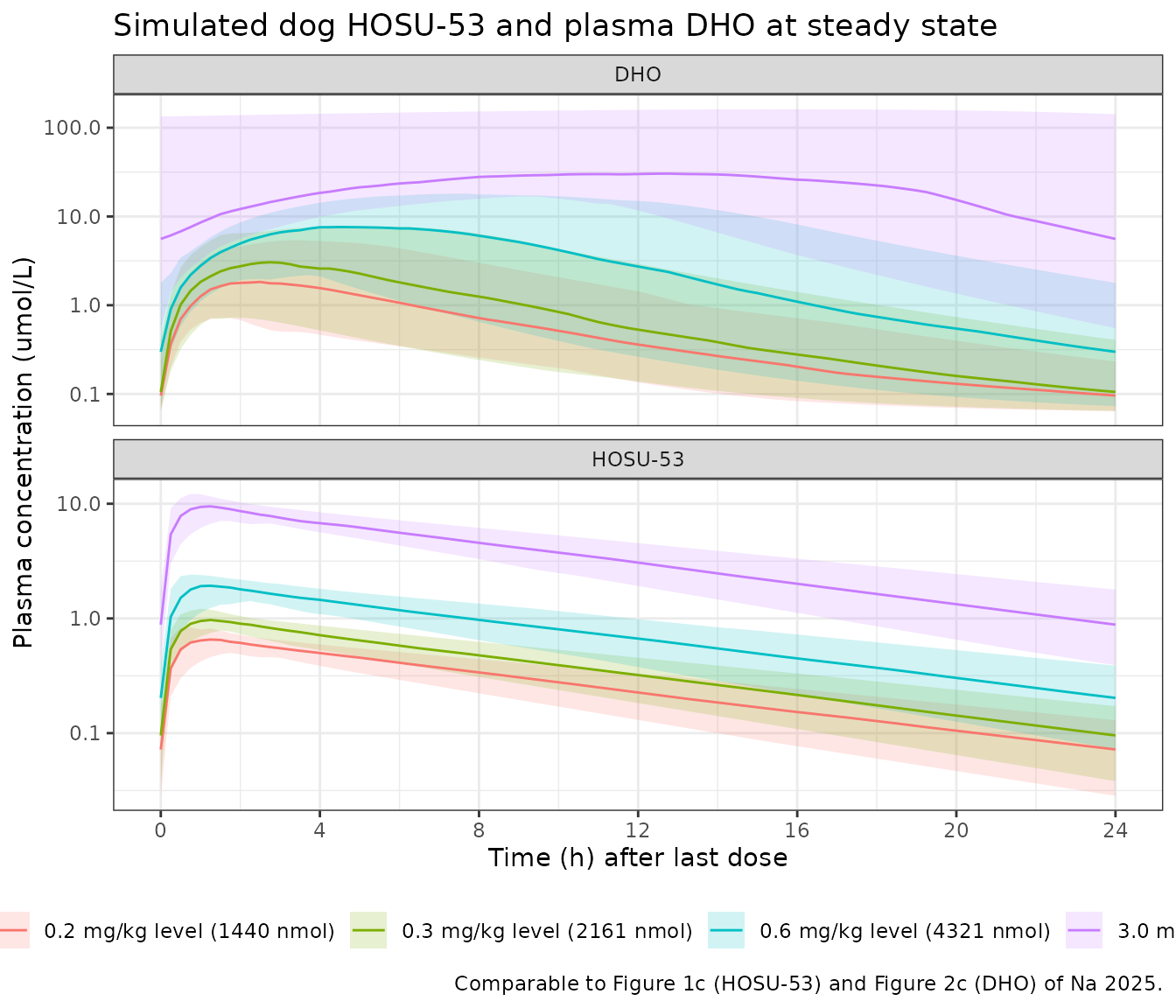
mouse_sim |>
  dplyr::filter(time >= 144, time <= 168) |>
  dplyr::mutate(tald = time - 144) |>
  dplyr::group_by(treatment, tald) |>
  dplyr::summarise(
    Q05 = stats::quantile(Cc, 0.05), Q50 = stats::quantile(Cc, 0.50),
    Q95 = stats::quantile(Cc, 0.95), .groups = "drop"
  ) |>
  ggplot(aes(tald, Q50, colour = treatment, fill = treatment)) +
  geom_ribbon(aes(ymin = Q05, ymax = Q95), alpha = 0.18, colour = NA) +
  geom_line() +
  scale_y_log10() +
  labs(x = "Time (h) after last dose", y = "HOSU-53 (umol/L)",
       colour = "Dose", fill = "Dose",
       title = "Simulated mouse HOSU-53 at steady state",
       caption = "Comparable to Supplementary Figure S1c of Na 2025.") +
  theme_bw() +
  theme(legend.position = "bottom")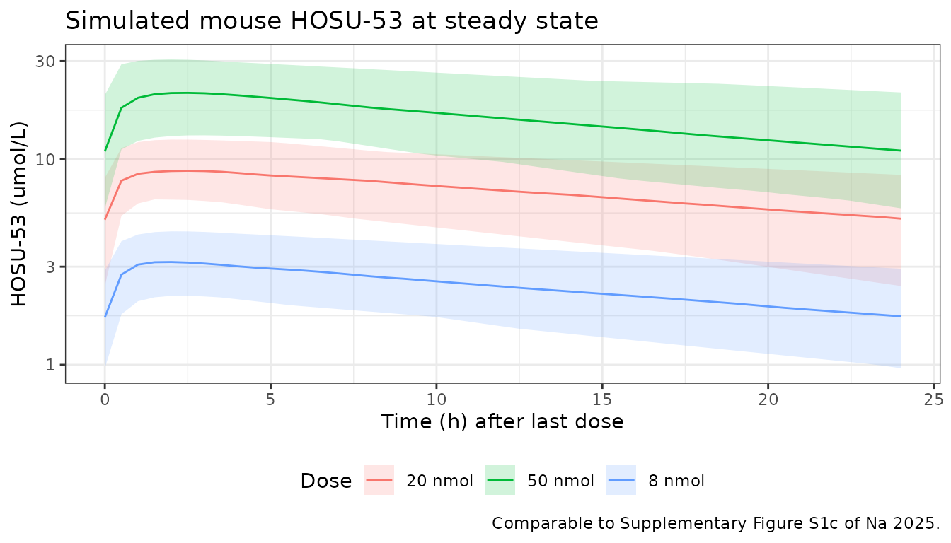
PKNCA validation
Na 2025 Section 3.2 reports the non-compartmental results the models must be consistent with: a mean elimination half-life of 6-8 h in dogs and 30 h in mice after a single IV (3 mg/kg) and oral (10 mg/kg) dose, with mean bioavailability of about 50% in dogs and 86% in mice. The NCA below is run on typical-value single-dose profiles for each species and route.
single_dose <- function(mod, amt, tmax, route, species) {
  s <- solve_typical(mod, add_obs(
    rxode2::et(amt = amt, cmt = if (route == "IV") "central" else "depot"),
    seq(0, tmax, by = tmax / 400)))
  data.frame(id = 1L, time = s$time, Cc = s$Cc,
             treatment = paste(species, route), amt = amt)
}

nca_conc <- dplyr::bind_rows(
  single_dose(dog_mod,   20000, 100, "IV", "dog"),
  single_dose(dog_mod,   20000, 100, "PO", "dog"),
  single_dose(mouse_mod, 20,    336, "IV", "mouse"),
  single_dose(mouse_mod, 20,    336, "PO", "mouse")
) |>
  dplyr::filter(!is.na(Cc)) |>
  # Per profile, keep Cc >= 1e-6 * Cmax after the peak: below that the ODE integrator has no relative accuracy left.
  dplyr::group_by(treatment, id) |>
  dplyr::filter(time == 0 | time <= time[which.max(Cc)] | Cc >= 1e-6 * max(Cc)) |>
  dplyr::ungroup()

# Time-zero guarantee (extravascular pre-dose Cc = 0).
nca_conc <- dplyr::bind_rows(
  nca_conc,
  nca_conc |> dplyr::distinct(id, treatment, amt) |> dplyr::mutate(time = 0, Cc = 0)
) |>
  dplyr::distinct(treatment, id, time, .keep_all = TRUE) |>
  dplyr::arrange(treatment, id, time)

conc_obj <- PKNCA::PKNCAconc(nca_conc, Cc ~ time | treatment + id)
dose_obj <- PKNCA::PKNCAdose(
  nca_conc |> dplyr::distinct(treatment, id, amt) |> dplyr::mutate(time = 0),
  amt ~ time | treatment + id
)
intervals <- data.frame(
  start = 0, end = Inf,
  cmax = TRUE, tmax = TRUE, auclast = TRUE, aucinf.obs = TRUE, half.life = TRUE
)
nca_res <- PKNCA::pk.nca(PKNCA::PKNCAdata(conc_obj, dose_obj, intervals = intervals))
nca_wide <- as.data.frame(nca_res) |>
  dplyr::filter(PPTESTCD %in% c("cmax", "tmax", "auclast", "aucinf.obs", "half.life")) |>
  dplyr::select(treatment, PPTESTCD, PPORRES) |>
  tidyr::pivot_wider(names_from = PPTESTCD, values_from = PPORRES)
nca_wide |> knitr::kable(digits = 3, caption = "PKNCA results on the typical-value single-dose profiles.")| treatment | auclast | cmax | tmax | half.life | aucinf.obs |
|---|---|---|---|---|---|
| dog IV | 133.361 | 20.408 | 0.00 | 7.087 | 133.368 |
| dog PO | 89.215 | 8.325 | 1.25 | 7.094 | 89.220 |
| mouse IV | 286.591 | 16.667 | 0.00 | 24.023 | 286.609 |
| mouse PO | 150.926 | 3.990 | 2.52 | 24.029 | 150.936 |
Comparison against published NCA
published <- tibble::tribble(
  ~treatment,  ~half.life,
  "dog IV",    7.0,     # Section 3.2: "mean elimination half-life (T1/2) of 6 to 8 h" (rats and dogs)
  "dog PO",    7.0,
  "mouse IV", 30.0,     # Section 3.2: "a longer mean T1/2 of 30 h" (mice)
  "mouse PO", 30.0
)

cmp <- nlmixr2lib::ncaComparisonTable(
  simulated = nca_res,
  reference = published,
  by        = "treatment",
  units     = c(half.life = "h"),
  tolerance_pct = 20
)
knitr::kable(cmp, caption = "Simulated vs. published half-life. * differs from reference by >20%.")| NCA parameter | treatment | Reference | Simulated | % diff |
|---|---|---|---|---|
| t½ (h) | dog IV | 7 | 7.09 | +1.2% |
| t½ (h) | dog PO | 7 | 7.09 | +1.3% |
| t½ (h) | mouse IV | 30 | 24 | -19.9% |
| t½ (h) | mouse PO | 30 | 24 | -19.9% |
The dog model returns a terminal half-life of 7.1 h, inside the 6-8 h range Na 2025 reports for dogs.
The mouse model returns 24.0 h against the reported mean NCA
half-life of 30 h – about 20% short, right at the flagging tolerance.
This is a property of the published parameters, not of the extraction:
log(2)/beta computed analytically from the Table S3 values
of CL, V1, Q, and V2 is 24.0 h, which the simulation reproduces to four
significant figures. The 30 h figure is a mean NCA value from the
single-dose study, whereas Table S3 is a simultaneous PK/PD SAEM fit
pooling three studies. Na 2025 itself flags the mouse half-life as the
anomaly in the dataset (Section 4: mouse elimination was much slower
than in rats and dogs, possibly through higher plasma protein binding,
and “this did not fully explain the PK differences in mice”). No
parameter was adjusted.
Bioavailability against the published NCA estimate
F is a structural parameter rather than an NCA
parameter, so it is compared separately.
f_from_nca <- function(sp) {
  po <- nca_wide$aucinf.obs[nca_wide$treatment == paste(sp, "PO")]
  iv <- nca_wide$aucinf.obs[nca_wide$treatment == paste(sp, "IV")]
  stopifnot(length(po) == 1L, length(iv) == 1L)
  po / iv
}
tibble::tibble(
  Species                      = c("dog", "mouse"),
  `Model F (Table 3 / S3)`     = c(0.67, 0.53),
  `F recovered from simulated AUC` = c(f_from_nca("dog"), f_from_nca("mouse")),
  `Published NCA F (Section 3.2)`  = c(0.50, 0.86)
) |>
knitr::kable(digits = 3, caption = "Bioavailability: model parameter, simulated AUC ratio, and the paper's own NCA estimate.")| Species | Model F (Table 3 / S3) | F recovered from simulated AUC | Published NCA F (Section 3.2) |
|---|---|---|---|
| dog | 0.67 | 0.669 | 0.50 |
| mouse | 0.53 | 0.527 | 0.86 |
The packaged models reproduce their own F exactly. The
population estimates differ from the paper’s NCA-derived values in
opposite directions (dog 0.67 vs about 0.50; mouse 0.53 vs 0.86). This
is a discrepancy within Na 2025, not an extraction
error: the NCA figures come from the single initial 10 mg/kg PO / 3
mg/kg IV study in 40% HPBCD, while the population estimates pool every
study, salt form, and vehicle. No parameter was tuned.
Dose proportionality in dogs
Na 2025 Section 3.2 reports that dog exposure “increased in a dose-proportional manner” over 0.3-3 mg/kg. Linear elimination makes this exact, which is a useful regression guard on the model file.
dose_prop <- dog_arms |>
  dplyr::rowwise() |>
  dplyr::mutate(
    auc24_ss = {
      s <- solve_typical(dog_mod, add_obs(
        rxode2::et(amt = amt, cmt = "depot", ii = 24, addl = 5L),
        seq(120, 144, by = 0.1)))
      trap_auc(s$time, s$Cc)
    }
  ) |>
  dplyr::ungroup() |>
  dplyr::mutate(dose_normalised_auc = auc24_ss / amt)

stopifnot(diff(range(dose_prop$dose_normalised_auc)) <
            1e-6 * mean(dose_prop$dose_normalised_auc))
dose_prop |>
  dplyr::select(treatment, auc24_ss, dose_normalised_auc) |>
  dplyr::rename("Dose arm" = treatment,
                "AUC(0-24,ss) (umol*h/L)" = auc24_ss,
                "Dose-normalised AUC" = dose_normalised_auc) |>
knitr::kable(digits = 6, caption = "Dog steady-state AUC is exactly dose-proportional.")| Dose arm | AUC(0-24,ss) (umol*h/L) | Dose-normalised AUC |
|---|---|---|
| 0.2 mg/kg level (1440 nmol) | 6.430740 | 0.004466 |
| 0.3 mg/kg level (2161 nmol) | 9.650571 | 0.004466 |
| 0.6 mg/kg level (4321 nmol) | 19.296683 | 0.004466 |
| 3.0 mg/kg level (21606 nmol) | 96.487903 | 0.004466 |
Na 2025 reports less-than-dose-proportional exposure in mice over 4-30 mg/kg (Section 3.2), which a linear-elimination model cannot reproduce; the mouse model was nevertheless fitted only over 3-10 mg/kg, where the linear assumption holds.
DHO exposure and the toxicity threshold
The paper’s central translational claim (Sections 3.2 and 4) is that
severe toxicity occurred in every species once the steady-state plasma
DHO exposure AUCtau,ss exceeded 1000 umolh/L, that the
optimal efficacy window is roughly 300-1000 umolh/L, and that the
highest DHO concentration observed without toxicity in
dogs was about 5850 ng/mL (37.0 umol/L). The dog model must place that
anchored exposure below the toxicity threshold.
dho_exposure <- function(mod, amt, ndose = 6L) {
  s <- solve_typical(mod, add_obs(
    rxode2::et(amt = amt, cmt = "depot", ii = 24, addl = ndose - 1L),
    seq(24 * (ndose - 1L), 24 * ndose, by = 0.05)))
  data.frame(amt = amt, dho_cmax = max(s$dho),
             dho_auctau = trap_auc(s$time, s$dho))
}
dog_dho <- dplyr::bind_rows(lapply(dog_arms$amt, function(a) dho_exposure(dog_mod, a))) |>
  dplyr::mutate(treatment = dog_arms$treatment)

anchored <- dog_dho[nrow(dog_dho), ]
stopifnot(
  abs(anchored$dho_cmax - dho_target) < 0.02 * dho_target, # anchor solved correctly
  anchored$dho_auctau < 1000,                              # non-toxic per Section 4
  anchored$dho_auctau > 300                                # inside the efficacy window
)

dog_dho |>
  dplyr::select(treatment, dho_cmax, dho_auctau) |>
  dplyr::rename("Dose arm" = treatment,
                "DHO Cmax,ss (umol/L)" = dho_cmax,
                "DHO AUCtau,ss (umol*h/L)" = dho_auctau) |>
  knitr::kable(digits = 1,
caption = "Simulated steady-state plasma DHO exposure in dogs. The toxicity threshold is 1000 umol*h/L and the efficacy window is 300-1000 umol*h/L (Na 2025 Sections 3.2 and 4).")| Dose arm | DHO Cmax,ss (umol/L) | DHO AUCtau,ss (umol*h/L) |
|---|---|---|
| 0.2 mg/kg level (1440 nmol) | 2.0 | 13.7 |
| 0.3 mg/kg level (2161 nmol) | 3.5 | 26.6 |
| 0.6 mg/kg level (4321 nmol) | 8.2 | 78.3 |
| 3.0 mg/kg level (21606 nmol) | 37.0 | 625.5 |
At the anchored top arm the model predicts a DHO
AUCtau,ss of 626 umolh/L – inside the paper’s stated
300-1000 umolh/L therapeutic window and below the 1000 umol*h/L
toxicity threshold, consistent with Na 2025’s report that no toxicity
accompanied the 5850 ng/mL maximum DHO observation.
threshold_amt <- stats::uniroot(
  function(a) dho_exposure(dog_mod, a)$dho_auctau - 1000,
  interval = c(dog_top_amt, 4 * dog_top_amt), tol = 50
)$root
c(anchored_top_dose_nmol = dog_top_amt,
  threshold_dose_nmol    = threshold_amt,
  fold_margin            = threshold_amt / dog_top_amt)
#> anchored_top_dose_nmol    threshold_dose_nmol            fold_margin
#>           21606.217104           29156.705141               1.349459
The 1000 umol*h/L threshold is crossed at only 1.35-fold the anchored
top arm. The steepness comes from the gamma of 1.9 combined
with the near-zero residual degradation once Cc is far
above the 0.1 umol/L IC50: DHO accumulation goes from
partially cleared to production-limited over a narrow dose band. That is
the same narrow margin Na 2025 describes clinically, where the dog NOAEL
of 0.6 mg/kg once daily sits one dose level below the adverse 1 mg/kg
once-daily arm.
Species comparison of the PD parameters
tibble::tibble(
  Parameter = c("R0 (umol/L)", "Kout (1/h)", "kin = R0*Kout (umol/L/h)",
                "IC50 (umol/L)", "gamma"),
  Dog   = c(0.06, 52, 0.06 * 52, 0.10, 1.90),
  Mouse = c(0.01, 155, 0.01 * 155, 1.55, 1.71)
) |>
  dplyr::mutate(`Mouse / dog` = Mouse / Dog) |>
knitr::kable(digits = 3, caption = "DHO turnover parameters by species (Na 2025 Table 3 and Table S3).")| Parameter | Dog | Mouse | Mouse / dog |
|---|---|---|---|
| R0 (umol/L) | 0.06 | 0.01 | 0.167 |
| Kout (1/h) | 52.00 | 155.00 | 2.981 |
| kin = R0*Kout (umol/L/h) | 3.12 | 1.55 | 0.497 |
| IC50 (umol/L) | 0.10 | 1.55 | 15.500 |
| gamma | 1.90 | 1.71 | 0.900 |
The Discussion states that the mouse and dog PD parameters “showed
overall comparability”. On the published numbers only the sigmoidicity
gamma is close (1.71 vs 1.90); the baseline R0
differs 6-fold, Kout 3-fold, and IC50 15-fold.
The values above are transcribed verbatim from Table 3 and Supplementary
Table S3 and were re-checked against the supplement PDF.
Assumptions and deviations
-
Dose-amount units are not published. Na 2025
reports volumes in mL and concentrations in umol/L but never states the
amount unit of its Monolix dataset, and does not report the HOSU-53
molecular weight. The model files declare
units$dosing = "nmol"because nmol / mL = umol/L is the only dimensionally consistent reading of the published tables. Converting a mg/kg dose into model units requires the unpublished molecular weight, so the dog arms in this vignette are anchored to the paper’s reported maximum observed dog DHO concentration (5850 ng/mL = 37.0 umol/L, Section 4) rather than stated in mg/kg. That anchoring additionally assumes the maximum observed DHO came from the highest included dog arm (3 mg/kg once daily), which Na 2025 does not state; the mg/kg labels on the simulated arms identify the published dose level each represents and are not a molecular-weight conversion. The mouse arms are given in model units only. Nothing in the model files depends on this anchoring – it affects only the illustrative dose scale in this vignette. -
One non-paper constant is used, and only in this
vignette. The 5850 ng/mL to 37.0 umol/L conversion above
divides by 158.11 g/mol, the standard molecular weight of dihydroorotic
acid (C5H6N2O4). That constant is not reported in Na 2025; it
is standard chemistry, introduced here solely to put the paper’s ng/mL
observation on the models’ umol/L scale. No parameter in either model
file depends on it. Na 2025 does contain one internal ng/mL to
micromolar pairing – Section 4’s “~25 uM DHO (or ~3200 ng/mL)”, quoted
for a different compound’s mouse study – which implies about 128 g/mol
and so disagrees with the true molecular weight by roughly 24%; both
numbers in that parenthetical are tilde-prefixed approximations, so it
is read as the paper rounding loosely rather than as a competing value.
The choice does not change any conclusion drawn here: re-anchoring the
dog arms with 128 g/mol instead of 158.11 raises the top arm’s DHO
AUCtau,ssfrom 626 to 826 umolh/L, which is still inside the paper’s 300-1000 umolh/L window and still below the 1000 umol*h/L toxicity threshold. -
dhoandDHOwere registered as new canonical compartment names. The plasma-dihydroorotate turnover state had no canonical name. Rather than declaring it per-paper,dho(the lowercase ODE state) andDHO(the uppercase observation-output sibling) were added toinst/references/compartment-names.mdunder Endogenous metabolic species, with these two model files as the founding examples, so that later DHODH-inhibitor extractions reuse the name. The lowercase-state / uppercase-observable split follows the registeredANC/ancandPRU/prupairs and is required becausecheckModelConventions()enforces lowercase ODE-state names. These models observe the lowercase state directly (dho ~ prop(propSd_dho)), which is equally permitted. -
The mouse half-life runs about 20% short of the published
NCA value. Analytically,
log(2)/betafrom the Table S3 disposition parameters is 24.0 h against the 30 h mean NCA half-life quoted in Section 3.2. The discrepancy is in the published numbers (a pooled three-study SAEM fit versus a single-study mean NCA), not in the transcription, and Na 2025 Section 4 already identifies mouse PK as the unexplained part of its dataset. No parameter was tuned. -
IIV is on the standard-deviation scale. Na 2025 was
fitted in Monolix, whose results table reports
omegaas the standard deviation of the random effect – the same scale as the “proportional residual error” rows of Table 3 and Table S3, which are the SD-scalebparameter of the Monolix error model. The paper does not say so explicitly.nlmixr2takes the variance, so each tabulated value is squared inini(). -
Imaxis fixed at 1. The final-model equation printed in Section 3.4 carries noImaxterm. The general form includingImaxappears only in Section 2.11 (human PD prediction).limax <- fixed(log(1))records this explicitly rather than dropping the term. -
CL/Fis encoded asCL. Table 3 and Table S3 label the clearance row “CL/F”, but both tables also reportFas a separate estimated parameter, and both fits used pooled IV and PO data (the dog disposition parameters came from an IV-only fit). The value is therefore a true clearance. The dimensional check supports this: the resulting terminal half-lives are 7.1 h (dog) and 24.0 h (mouse), matching the 6-8 h and 30 h NCA values in Section 3.2. Reading it asCL/Finstead would shorten both half-lives by a factor ofF. -
Qis in mL/h, not L/h. TheQrow header of Table 3 and Table S3 reads “Q (mL/h)”, but the abbreviation footnote of both tables reads “Q, intercompartment clearance (L/h)”. mL/h is the correct reading: it is the unit consistent withCLandV1in the same tables, 400 L/h is physiologically impossible in a dog, and only mL/h reproduces the published NCA half-lives. - No erratum applies. PubMed (PMID 40284407) and Europe PMC list no correction, corrigendum, or erratum for this article as of the extraction date.
-
No covariates. Sex, dose level, salt form, and
vehicle formulation were screened (Section 2.7) and none were retained
(Section 3.3). They are recorded in each model file’s
covariatesDataExcludedmetadata so the screen’s provenance survives, but they are absent frommodel(). - The rat model does not exist. Na 2025 Section 3.3 excluded the rat data from the population modelling because dose proportionality was not met.
- The PK-Sim PBPK models are not extracted. Na 2025 built whole-body PBPK models for rat, dog, and human in PK-Sim v11.0, but the only model inputs published are the compound-specific properties in Table 1 and Supplementary Table S2 (lipophilicity, fu, pKa, solubility, intestinal permeability, specific clearance, blood:plasma ratio). The physiological structure, organ volumes, blood flows, partition coefficients, and cellular permeabilities are supplied by the PK-Sim platform and are not written out in any available source, so the PBPK models are not reproducible here without substituting platform defaults. Table 4 (time above the 669 pM hepatic target) and Figure 3 (human plasma and hepatic profiles) are PBPK outputs and are likewise not reproduced.
-
The human PD prediction is not reproduced. Section
2.11 predicts human DHO by driving the dog PD parameters with the
PBPK-predicted human HOSU-53 plasma profile. That driving profile is a
PBPK output (see above), so the quoted human results – DHO Cmax of about
791 ng/mL at 5 mg and 5500 ng/mL at 25 mg, and an
AUCtau,ssof 623 umol*h/L at 25 mg once daily – cannot be regenerated from the packaged models alone. - The published pcVPCs are not prediction-corrected here. Figures 1c and 2c of Na 2025 are prediction-corrected VPCs against observed data that are not publicly available. The figures above show the simulated median and 5th/95th percentiles over the same time-after-last-dose window, which reproduces the concentration range and shape but not the correction.
-
Multi-endpoint event tables select the endpoint with
dvid. Both models carry two residual-error endpoints (Ccanddho), and rxode2 appends one pseudo-compartment per endpoint after the ODE states, then requires every observation row to select one of them. The selector is thedvidcolumn, notcmt: withdvidabsent, an observation row naming an ODE state fails with'dvid'->'cmt' or 'cmt' on observation record. Every event table here therefore keeps ODE-state names incmt(depot/central) on both dose and observation rows and addsdvid = 1Lon the observation rows. Selecting one endpoint is sufficient – rxSolve returns bothCcanddhoon those rows. Putting an algebraic observable name incmtalso runs, but it auto-injects a compartment slot for that observable and renumbers the ODE states, so it is avoided here. -
Baseline DHO relative to the assay. The dog
R0of 0.06 umol/L is essentially the dog DHO assay LLOQ of 10 ng/mL (0.063 umol/L), consistent with Section 3.1’s report that 21.3% of dog DHO samples – including pre-dose samples – were below quantification. The mouseR0of 0.01 umol/L (1.6 ng/mL) sits below the 10 ng/mL mouse assay LLOQ and is therefore an extrapolated baseline identified mainly by post-dose data. Both are used as published.