Recombinant Erwinia chrysanthemi asparaginase (Lin 2023)
Source:vignettes/articles/Lin_2023_asparaginaseErwiniaRecombinant.Rmd
Lin_2023_asparaginaseErwiniaRecombinant.Rmd
mod <- rxode2::rxode(readModelDb("Lin_2023_asparaginaseErwiniaRecombinant"))Model and source
- Citation: Lin T, Whigham T, Fernando I, Choi MR, Wang Q, Silverman JA. Population pharmacokinetics of intramuscular recombinant Erwinia chrysanthemi asparaginase (JZP458) in patients with acute lymphoblastic leukemia. Clin Transl Sci. 2023;16(5):898-909. doi:10.1111/cts.13499
- Description: One-compartment population PK model for intramuscular recombinant Erwinia chrysanthemi asparaginase (JZP458, marketed as Rylaze) in pediatric and young-adult patients with acute lymphoblastic leukemia or lymphoblastic lymphoma who developed hypersensitivity to E. coli-derived asparaginases (Lin 2023, phase II/III study AALL1931). The measured quantity is serum asparaginase activity (SAA), so all amounts are activity units (IU) rather than mass. Absorption is mixed-order: the dose enters the depot as a zero-order input at a constant rate R1, running simultaneously with first-order absorption Ka out of the depot, which makes the terminal phase absorption rate limited (flip-flop). Ka, R1 and the relative bioavailability F were fixed to values carried over from the phase I intensive-sampling PopPK model (Lin 2021) because the sparse AALL1931 sampling could not characterize the absorption phase. Body surface area is an allometric covariate on both clearance and volume; Black or African American race and T-cell ALL disease subtype are multiplicative fractional-change covariates on clearance. Interindividual variability is exponential on clearance and volume, with a combined proportional and additive residual error.
- Article: https://doi.org/10.1111/cts.13499
- Upstream phase I population PK model that supplied the three fixed absorption parameters: https://doi.org/10.1002/cpdd.1002
- Upstream phase I study reporting the noncompartmental analysis, cited as reference 16 of Lin 2023 and not used as a source here: Lin T, Hernandez-Illas M, Rey A, et al. Clin Transl Sci. 2021;14:870-879.
JZP458 (marketed as Rylaze) is a recombinant Erwinia chrysanthemi asparaginase produced in a Pseudomonas fluorescens expression platform. It is given to patients with acute lymphoblastic leukemia (ALL) or lymphoblastic lymphoma (LBL) who have developed hypersensitivity to E. coli-derived asparaginases. The measured quantity is serum asparaginase activity (SAA), and the therapeutic target is a nadir SAA (NSAA) of at least 0.1 IU/mL, the accepted threshold for adequate asparagine depletion.
Population
The model was fit to 2687 SAA observations (2145 quantifiable, 542 below the limit of quantitation, handled by the Beal M3 method) from 166 patients in the phase II/III AALL1931 study (NCT04145531), run with the Children’s Oncology Group. Patients were 1.7 to 25 years old (mean 10.2, median 10.0 years), weighed 9.33 to 131.0 kg (median 36.5 kg), and had a body surface area of 0.44 to 2.53 m^2 (mean 1.23, median 1.17 m^2). 38.0% were female. Race was 68.7% White/Caucasian, 13.3% Black/African American, 4.2% Asian, 1.8% American Indian/Alaska Native, 0.6% Other and 11.4% declined to state; 31.3% were Hispanic or Latino. Primary disease was ALL in 89.8% and LBL in 10.2%, with disease subtype B-ALL 74.1%, T-ALL 15.7%, T-LBL 9.6% and B-LBL 0.6%. All 166 patients had received pegaspargase before study entry, and exactly half were antidrug-antibody positive. Three intramuscular Monday/Wednesday/Friday cohorts were enrolled: 25 mg/m^2 (n = 32), 37.5 mg/m^2 (n = 83) and 25/25/50 mg/m^2 (n = 51). Baseline demographics are Lin 2023 Table 1.
The same information is available programmatically from the model’s
population metadata:
str(mod$population, max.level = 1)
#> List of 16
#>  $ species       : chr "human"
#>  $ n_subjects    : int 166
#>  $ n_studies     : int 1
#>  $ n_observations: int 2687
#>  $ age_range     : chr "1.7-25 years"
#>  $ age_median    : chr "10.0 years"
#>  $ weight_range  : chr "9.33-131.0 kg"
#>  $ weight_median : chr "36.5 kg"
#>  $ bsa_range     : chr "0.44-2.53 m^2"
#>  $ bsa_median    : chr "1.17 m^2"
#>  $ sex_female_pct: num 38
#>  $ race_ethnicity: Named num [1:6] 68.7 13.3 4.2 1.8 0.6 11.4
#>   ..- attr(*, "names")= chr [1:6] "White/Caucasian" "Black/African American" "Asian" "American Indian/Alaska Native" ...
#>  $ disease_state : chr "Newly diagnosed acute lymphoblastic leukemia (89.8%) or lymphoblastic lymphoma (10.2%) with a grade 3 or greate"| __truncated__
#>  $ dose_range    : chr "Intramuscular JZP458 in three Monday/Wednesday/Friday cohorts: 25 mg/m^2 (n = 32), 37.5 mg/m^2 (n = 83) and 25/"| __truncated__
#>  $ regions       : chr "Children's Oncology Group sites (AALL1931; NCT04145531)"
#>  $ notes         : chr "Lin 2023 Table 1 (baseline demographics of the PopPK analysis set) and Results, Patient demographics. 2687 SAA "| __truncated__
Source trace
Every ini() entry in
inst/modeldb/specificDrugs/Lin_2023_asparaginaseErwiniaRecombinant.R
carries an in-file comment naming its origin. They are collected here
for review.
| Equation / parameter | Value | Source location |
|---|---|---|
lcl (CL) |
146 mL/h | Lin 2023 Table 2 (SE 4.93, RSE 3.38%, 95% CI 136-156) |
lvc (V) |
445 mL | Lin 2023 Table 2 (SE 34.9, RSE 7.85%, 95% CI 377-513) |
lka (Ka) |
0.0369 1/h, fixed | Lin 2023 Table 2 (no SE/RSE/CI); fixed from the phase I model of Lin 2021 |
lr1 (R1) |
1810 IU/h, fixed | Lin 2023 Table 2 (no SE/RSE/CI); fixed from the phase I model of Lin 2021 |
lfdepot (F) |
0.359, fixed | Lin 2023 Table 2 (no SE/RSE/CI); fixed from the phase I model of Lin 2021 |
e_bsa_cl |
1.48 | Lin 2023 Table 2 (SE 0.0686, RSE 4.63%, 95% CI 1.35-1.61) |
e_bsa_vc |
1.61 | Lin 2023 Table 2 (SE 0.151, RSE 9.4%, 95% CI 1.31-1.91) |
e_black_cl |
0.674 | Lin 2023 Table 2 (SE 0.0715, RSE 10.6%, 95% CI 0.534-0.814) |
e_tall_cl |
0.771 | Lin 2023 Table 2 (SE 0.0686, RSE 8.89%, 95% CI 0.637-0.905) |
etalcl |
0.125 (CV 36.5%) | Lin 2023 Table 2 (SE 0.0173, RSE 13.8%, 95% CI 0.0911-0.159) |
etalvc |
0.479 (CV 78.4%) | Lin 2023 Table 2 (SE 0.0867, RSE 18.1%, 95% CI 0.309-0.649) |
propSd |
0.46 | Lin 2023 Table 2 (SE 0.00665, RSE 1.45%, 95% CI 0.447-0.473) |
addSd |
0.0166 IU/mL | Lin 2023 Table 2 (SE 0.000539, RSE 3.25%, 95% CI 0.0155-0.0177) |
| CL covariate equation | 146 * (BSA/1.2)^1.48 * 0.674^BLACK * 0.771^TALL |
Lin 2023 Results, Covariate analysis and final PopPK model selection (printed equation) |
| V covariate equation | 445 * (BSA/1.2)^1.61 |
Lin 2023 Results, Covariate analysis and final PopPK model selection (printed equation) |
| BSA reference 1.2 m^2 | n/a | Lin 2023 Results, Base model (“The BSA standard used for scaling was 1.2 m^2”) |
| Mixed-order absorption structure | n/a | Lin 2023 Results, Base model; Discussion; Lin 2021 Results, Base model |
| One-compartment linear elimination | n/a | Lin 2023 Results, Base model |
| Proportional + additive residual error | n/a | Lin 2023 Table 2 and Results, Base model |
The ini() values reconcile with Table 2’s own CV column,
which is a useful check that the Estimate column holds variances rather
than standard deviations:
Model structure
One compartment with linear elimination and simultaneous
mixed-order absorption: the dose enters the depot
as a zero-order input running at the constant rate R1,
while first-order absorption Ka drains the depot into
central at the same time. Lin 2023 (Results, Base model)
describes it as “simultaneous mixed-order absorption (zero-order
infusion followed by a first-order absorption)”; the upstream Lin 2021
calls the same construct a “sequential mixed order absorption function”.
R1 is the NONMEM reserved zero-order input rate for the
dosing compartment, so the input duration is
F * amt / R1.
Because Ka (0.0369 /h) is roughly nine times smaller
than kel = CL/V (0.328 /h at the reference BSA),
disposition is absorption rate limited (flip-flop) and
the terminal slope reports Ka, not kel.
Dose records must set rate = -1
rxode2 only consults a modelled rate() when the dose
record asks for it. With the default rate = 0 the modelled
rate is silently ignored and the dose is delivered as
an instantaneous bolus into the depot. The check below documents the
difference so the requirement is visible rather than folklore.
tv <- rxode2::zeroRe(mod)

solve_one <- function(dose, rate, bsa = 1.2, black = 0, tall = 0,
                      times = seq(0, 240, by = 0.05), ii = 0, addl = 0) {
  ev <- rxode2::et(amt = dose, cmt = "depot", rate = rate, ii = ii, addl = addl) |>
    rxode2::et(times, cmt = "central")
  ev <- as.data.frame(ev)
  ev$BSA <- bsa; ev$RACE_BLACK <- black; ev$DIS_TALL <- tall
  out <- rxode2::rxSolve(tv, ev, returnType = "data.frame")
  if (is.null(out$id)) out$id <- 1L
  out[!is.na(out$Cc), ]
}

probe_dose <- 20000                       # IU; see "Dose units" below
s_rate  <- solve_one(probe_dose, rate = -1)
#> ℹ omega/sigma items treated as zero: 'etalcl', 'etalvc'
s_bolus <- solve_one(probe_dose, rate = 0)
#> ℹ omega/sigma items treated as zero: 'etalcl', 'etalvc'

dur_expected <- exp(mod$theta[["lfdepot"]]) * probe_dose / exp(mod$theta[["lr1"]])
ka_i  <- exp(mod$theta[["lka"]])
kel_i <- 146 / 445
tmax_bolus_expected <- log(kel_i / ka_i) / (kel_i - ka_i)

rate_check <- data.frame(
  Quantity = c("depot peak time (h)", "Tmax of Cc (h)", "Cmax (IU/mL)"),
  `rate = -1` = c(s_rate$time[which.max(s_rate$depot)],
                  s_rate$time[which.max(s_rate$Cc)],
                  max(s_rate$Cc)),
  `rate = 0` = c(s_bolus$time[which.max(s_bolus$depot)],
                 s_bolus$time[which.max(s_bolus$Cc)],
                 max(s_bolus$Cc)),
  check.names = FALSE
)
knitr::kable(rate_check, digits = 3,
caption = "Modelled zero-order rate is active only with rate = -1.")| Quantity | rate = -1 | rate = 0 |
|---|---|---|
| depot peak time (h) | 4.000 | 0.000 |
| Tmax of Cc (h) | 9.700 | 7.500 |
| Cmax (IU/mL) | 1.365 | 1.376 |
sprintf("expected zero-order duration F*amt/R1 = %.3f h", dur_expected)
#> [1] "expected zero-order duration F*amt/R1 = 3.967 h"
sprintf("expected bolus Tmax log(kel/ka)/(kel-ka) = %.3f h", tmax_bolus_expected)
#> [1] "expected bolus Tmax log(kel/ka)/(kel-ka) = 7.504 h"

# Deterministic identities, so these are asserted tightly.
stopifnot(
  abs(s_rate$time[which.max(s_rate$depot)] - dur_expected) < 0.06,
  abs(s_bolus$time[which.max(s_bolus$Cc)] - tmax_bolus_expected) < 0.06,
  s_bolus$time[which.max(s_bolus$depot)] == 0
)
Note that Cmax differs by well under 1% between the two,
so Cmax alone will not reveal the mistake – only the
depot peak time and Tmax do.
Dose units: activity units, not mass
The model’s amount unit is IU of asparaginase activity, not
mg. Two independent facts in the sources force this reading:
the zero-order absorption rate is reported in IU/h (Lin
2023 Table 2; Lin 2021 Table 2), and the observation
Cc = central / vc is only IU/mL if central is
in IU.
Neither Lin 2023 nor its upstream Lin 2021 states the mg-to-IU specific activity of JZP458. A clinical dose of 25 mg/m^2 therefore cannot be converted into model units from any published source, and no conversion factor is baked into the model file. Dose this model in IU.
The primary validation below is built entirely from dose-independent published quantities, so it does not depend on resolving this gap. A reconstruction of the dose scale is given afterwards, clearly separated and flagged as not a published value.
Validation 1: dose-independent post-hoc parameters
Lin 2023 (Results, Covariate analysis and final PopPK model
selection) reports three post-hoc quantities that do not depend on the
dose scale: the geometric mean apparent clearance CL/F of
0.31 L/h/m^2, apparent volume V/F of 1.14 L/m^2, and
terminal half-life t1/2 of 19.1 h. CL/F and
V/F follow by arithmetic from Table 2; t1/2 is
recovered from the simulated terminal slope.
bsa_ref <- 1.2
cl_ref  <- exp(mod$theta[["lcl"]])
vc_ref  <- exp(mod$theta[["lvc"]])
f_ref   <- exp(mod$theta[["lfdepot"]])

clf_per_m2 <- cl_ref / f_ref / bsa_ref / 1000   # mL/h -> L/h, then per m^2
vf_per_m2  <- vc_ref / f_ref / bsa_ref / 1000   # mL   -> L,   then per m^2

# Terminal slope taken well after the input has stopped, so it reports ka.
# Keep Cc >= 1e-6 * max(Cc): below that the ODE solution is integrator noise.
tail_s  <- s_rate[s_rate$time >= 150 & s_rate$time <= 240 &
                    s_rate$Cc >= 1e-6 * max(s_rate$Cc), ]
slope   <- stats::coef(stats::lm(log(tail_s$Cc) ~ tail_s$time))[[2]]
thalf   <- log(2) / (-slope)

posthoc <- data.frame(
  Quantity  = c("CL/F (L/h/m^2)", "V/F (L/m^2)", "Terminal t1/2 (h)"),
  Model     = c(clf_per_m2, vf_per_m2, thalf),
  Published = c(0.31, 1.14, 19.1)
)
posthoc$`Difference (%)` <- 100 * (posthoc$Model - posthoc$Published) / posthoc$Published
knitr::kable(posthoc, digits = 3,
caption = "Model versus the post-hoc values reported by Lin 2023.")| Quantity | Model | Published | Difference (%) |
|---|---|---|---|
| CL/F (L/h/m^2) | 0.339 | 0.31 | 9.324 |
| V/F (L/m^2) | 1.033 | 1.14 | -9.389 |
| Terminal t1/2 (h) | 18.784 | 19.10 | -1.652 |
The half-life is the sharpest of the three: it is a pure statement
that the terminal phase is absorption rate limited, and
log(2)/Ka = 18.78 h reproduces the published 19.1 h to
within 2%. Lin 2023 reports only a 3% CV on the individual
t1/2 values, which is itself evidence that Ka
was fixed rather than estimated. CL/F and V/F
are geometric means over a population whose BSA is normalised linearly
in the paper’s summary but enters the model as BSA^1.48 and
BSA^1.61, so a few percent of disagreement is expected.
Validation 2: exact covariate identities
The covariate model is multiplicative and acts only on clearance and volume, so each published coefficient must reproduce exactly as a ratio of typical-value exposures. These are deterministic, so they are asserted to solver tolerance.
auc_of <- function(bsa, black, tall) {
  s <- solve_one(probe_dose, rate = -1, bsa = bsa, black = black, tall = tall,
                 times = seq(0, 600, by = 0.25))
  sum(diff(s$time) * (utils::head(s$Cc, -1) + utils::tail(s$Cc, -1)) / 2)
}
auc_ref <- auc_of(1.2, 0, 0)
#> ℹ omega/sigma items treated as zero: 'etalcl', 'etalvc'

cov_check <- data.frame(
  Comparison = c("Black/African American vs reference",
                 "T-ALL vs reference",
                 "BSA 2.4 vs 1.2 m^2 (dose held fixed)"),
  Observed = c(auc_of(1.2, 1, 0) / auc_ref,
               auc_of(1.2, 0, 1) / auc_ref,
               auc_of(2.4, 0, 0) / auc_ref),
  Expected = c(1 / 0.674, 1 / 0.771, 2^-1.48)
)
#> ℹ omega/sigma items treated as zero: 'etalcl', 'etalvc'
#> ℹ omega/sigma items treated as zero: 'etalcl', 'etalvc'
#> ℹ omega/sigma items treated as zero: 'etalcl', 'etalvc'
knitr::kable(cov_check, digits = 5,
caption = "Exposure ratios reproduce the published coefficients.")| Comparison | Observed | Expected |
|---|---|---|
| Black/African American vs reference | 1.48368 | 1.48368 |
| T-ALL vs reference | 1.29702 | 1.29702 |
| BSA 2.4 vs 1.2 m^2 (dose held fixed) | 0.35849 | 0.35849 |
The AUC ratio is 1/0.674 and 1/0.771 rather
than 0.674 and 0.771 because these
coefficients act on clearance, and AUC is inversely
proportional to clearance. The BSA row confirms the 1.48 exponent:
holding the dose fixed, doubling BSA divides exposure by
2^1.48. Because the clinical dose is itself
BSA-proportional, the net effect of larger BSA on exposure is
BSA^(1 - 1.48) = BSA^-0.48 – a mild decrease,
which is why the paper’s smallest patients are not the ones at risk of
missing the NSAA target.
Validation 3: PKNCA on the typical-value profile
NCA is run on the typical-value (no IIV, no residual error)
single-dose profile. Running it over a full-IIV cohort would make the
half-life estimate both NA-poisoned and Tmax-selected, which is not what
the published t1/2 means.
nca_in <- s_rate |>
  dplyr::filter(!is.na(Cc)) |>
  dplyr::select(id, time, Cc) |>
  # Keep Cc >= 1e-6 * max(Cc) after the peak (solver noise below), plus the time-zero anchor.
  dplyr::filter(time <= time[which.max(Cc)] | Cc >= 1e-6 * max(Cc) | time == 0)

# Defensive time-zero record so PKNCA does not warn about an AUC range
# starting before the first measurement.
if (!any(nca_in$time == 0)) {
  nca_in <- dplyr::bind_rows(
    data.frame(id = 1L, time = 0, Cc = 0), nca_in
  ) |> dplyr::distinct(id, time, .keep_all = TRUE) |> dplyr::arrange(time)
}

dose_df <- data.frame(id = 1L, time = 0, amt = probe_dose)

o_conc <- PKNCA::PKNCAconc(nca_in, Cc ~ time | id)
o_dose <- PKNCA::PKNCAdose(dose_df, amt ~ time | id)
o_data <- PKNCA::PKNCAdata(
  o_conc, o_dose,
  intervals = data.frame(
    start = 0, end = 240,
    cmax = TRUE, tmax = TRUE, half.life = TRUE,
    auclast = TRUE, aucinf.obs = TRUE
  )
)
res <- as.data.frame(PKNCA::pk.nca(o_data))
knitr::kable(res[, c("PPTESTCD", "PPORRES")], digits = 4,
caption = "PKNCA summary of the typical-value single-dose profile.")| PPTESTCD | PPORRES |
|---|---|
| auclast | 49.1696 |
| cmax | 1.3650 |
| tmax | 9.7000 |
| tlast | 240.0000 |
| clast.obs | 0.0003 |
| lambda.z | 0.0369 |
| r.squared | 1.0000 |
| adj.r.squared | 1.0000 |
| lambda.z.time.first | 9.7500 |
| lambda.z.time.last | 240.0000 |
| lambda.z.n.points | 4606.0000 |
| clast.pred | 0.0003 |
| half.life | 18.8067 |
| span.ratio | 12.2430 |
| aucinf.obs | 49.1781 |
get_nca <- function(code) res$PPORRES[res$PPTESTCD == code]
stopifnot(length(get_nca("half.life")) == 1L)   # guard: the lookup must hit

simulated <- data.frame(
  `t.5` = get_nca("half.life"),
  Tmax  = get_nca("tmax"),
  check.names = FALSE
)
reference <- data.frame(
  `t.5` = 19.1,
  Tmax  = 12.0,
  check.names = FALSE
)
knitr::kable(
  nlmixr2lib::ncaComparisonTable(
    simulated, reference,
    units = c(`t.5` = "h", Tmax = "h")
  ),
  caption = paste(
    "Typical-value NCA versus the median post-hoc values of Lin 2023.",
    "Tmax depends on the dose scale; see Errata."
  )
)
#> Warning: ncaParamLabel(): unknown PKNCA code(s) returned as-is: 't.5', 'Tmax'| NCA parameter | Reference | Simulated | % diff |
|---|---|---|---|
| t.5 (h) | 19.1 | 18.8 | -1.5% |
| Tmax (h) | 12 | 9.7 | -19.2% |
aucinf.obs equals auclast here because the
240 h window is roughly 13 absorption half-lives, so the extrapolated
tail is negligible; the identity is asserted as an inequality rather
than an equality.
Dose-scale reconstruction (not a published value)
Everything above is dose-independent. To simulate the clinical mg/m^2 regimens the missing mg-to-IU factor is needed, so this section reconstructs it from the paper’s own simulation output and labels the result clearly. It is not a published number and is not part of the model file.
Lin 2023 Figure 3b plots the simulated median SAA profile for 25 mg/m^2 every 48 h in the NHANES virtual population (median BSA 1.66 m^2). Reading the first peak off that figure at about 1.0 IU/mL fixes the scale; the steady-state peak, the trough and Tmax are then held-out landmarks that the reconstruction was not fitted to.
bsa_nhanes <- 1.66
mgm2       <- 25

first_peak_target <- 1.0   # digitised from Lin 2023 Figure 3b

sim_regimen <- function(dose_iu, bsa) {
  solve_one(dose_iu, rate = -1, bsa = bsa,
            times = seq(0, 336, by = 0.25), ii = 48, addl = 6)
}
obj <- function(dose_iu) {
  s <- sim_regimen(dose_iu, bsa_nhanes)
  max(s$Cc[s$time <= 48]) - first_peak_target
}
dose_iu_recon <- stats::uniroot(obj, c(2000, 200000))$root
#> ℹ omega/sigma items treated as zero: 'etalcl', 'etalvc'
#> ℹ omega/sigma items treated as zero: 'etalcl', 'etalvc'
#> ℹ omega/sigma items treated as zero: 'etalcl', 'etalvc'
#> ℹ omega/sigma items treated as zero: 'etalcl', 'etalvc'
#> ℹ omega/sigma items treated as zero: 'etalcl', 'etalvc'
#> ℹ omega/sigma items treated as zero: 'etalcl', 'etalvc'
#> ℹ omega/sigma items treated as zero: 'etalcl', 'etalvc'
#> ℹ omega/sigma items treated as zero: 'etalcl', 'etalvc'
#> ℹ omega/sigma items treated as zero: 'etalcl', 'etalvc'
specific_activity <- dose_iu_recon / (mgm2 * bsa_nhanes)

sprintf("reconstructed specific activity ~ %.0f IU/mg (NOT a published value)",
        specific_activity)
#> [1] "reconstructed specific activity ~ 577 IU/mg (NOT a published value)"

s_rec <- sim_regimen(dose_iu_recon, bsa_nhanes)
#> ℹ omega/sigma items treated as zero: 'etalcl', 'etalvc'
landmarks <- data.frame(
  Landmark = c("first peak (fitted)", "steady-state peak (held out)",
               "trough before dose 7 (held out)", "Tmax of first dose (held out)"),
  Model = c(max(s_rec$Cc[s_rec$time <= 48]),
            max(s_rec$Cc[s_rec$time > 240 & s_rec$time < 290]),
            s_rec$Cc[which.min(abs(s_rec$time - 288))],
            s_rec$time[which.max(s_rec$Cc[s_rec$time <= 48])]),
  `Lin 2023` = c("~1.0 IU/mL (Figure 3b)", "~1.3 IU/mL (Figure 3b)",
                 "~0.35-0.40 IU/mL (Figure 3b)", "12.0 h median (Results text)"),
  check.names = FALSE
)
knitr::kable(landmarks, digits = 2,
caption = "Held-out landmarks the dose-scale fit was not calibrated to.")| Landmark | Model | Lin 2023 |
|---|---|---|
| first peak (fitted) | 1.00 | ~1.0 IU/mL (Figure 3b) |
| steady-state peak (held out) | 1.24 | ~1.3 IU/mL (Figure 3b) |
| trough before dose 7 (held out) | 0.34 | ~0.35-0.40 IU/mL (Figure 3b) |
| Tmax of first dose (held out) | 10.50 | 12.0 h median (Results text) |
ggplot2::ggplot(s_rec, ggplot2::aes(time, Cc)) +
  ggplot2::geom_line(colour = "steelblue") +
  ggplot2::geom_hline(yintercept = 0.1, linetype = "dashed") +
  ggplot2::scale_y_log10() +
  ggplot2::scale_x_continuous(breaks = seq(0, 336, by = 48)) +
  ggplot2::labs(
    x = "Time (hours)", y = "SAA (IU/mL)",
    title = "Typical-value SAA, 25 mg/m^2 every 48 h at BSA 1.66 m^2",
    subtitle = "Compare Lin 2023 Figure 3b (median of the NHANES virtual population)"
  ) +
  ggplot2::theme_bw()
#> Warning in ggplot2::scale_y_log10(): log-10 transformation introduced infinite
#> values.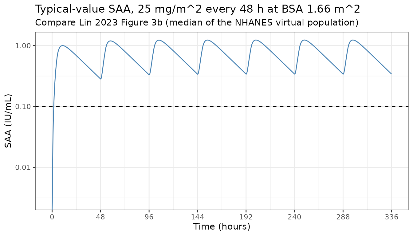
# Loose bounds: the target was read off a log-scale figure by eye, so the
# reconstruction carries perhaps 20-25% uncertainty. These bounds still go red
# on a mis-transcribed CL, V, Ka or R1, which move the landmarks severalfold.
stopifnot(
  specific_activity > 350, specific_activity < 900,
  max(s_rec$Cc[s_rec$time > 240 & s_rec$time < 290]) > 1.0,
  max(s_rec$Cc[s_rec$time > 240 & s_rec$time < 290]) < 1.7,
  s_rec$Cc[which.min(abs(s_rec$time - 288))] > 0.2,
  s_rec$Cc[which.min(abs(s_rec$time - 288))] < 0.6
)
The reconstruction lands near 580 IU/mg. It rests on a single value
read by eye off a base-10 log axis on which 1.00 is a printed gridline,
so it is worth perhaps one significant figure. No conversion
factor is committed to the model file: the specific activity of
JZP458 is a product attribute rather than a model parameter, it is
absent from every available source, and baking a figure-derived estimate
into ini() would give it a false precision. See Errata.
Virtual cohort
A 200-subject cohort matching the AALL1931 analysis-set covariate distributions is simulated on the 25 mg/m^2 every-48-h regimen, using the reconstructed dose scale. This is illustrative rather than a reproduction of the paper’s response rates, which were computed on the NHANES virtual population.
rxode2::rxSetSeed(20230501)
n_sub <- 200

set.seed(20230501)
cohort <- data.frame(
  id  = seq_len(n_sub),
  # Log-normal BSA matched to the analysis-set median 1.17 and range 0.44-2.53.
  BSA = pmin(pmax(stats::rlnorm(n_sub, log(1.17), 0.42), 0.44), 2.53),
  RACE_BLACK = stats::rbinom(n_sub, 1, 0.133),
  DIS_TALL   = stats::rbinom(n_sub, 1, 0.157)
)
cohort$amt <- mgm2 * cohort$BSA * specific_activity

ev_cohort <- lapply(seq_len(n_sub), function(i) {
  e <- rxode2::et(amt = cohort$amt[i], cmt = "depot", rate = -1,
                  ii = 48, addl = 6) |>
    rxode2::et(seq(0, 336, by = 2), cmt = "central")
  e <- as.data.frame(e)
  e$id <- cohort$id[i]
  e$BSA <- cohort$BSA[i]
  e$RACE_BLACK <- cohort$RACE_BLACK[i]
  e$DIS_TALL <- cohort$DIS_TALL[i]
  e
}) |> dplyr::bind_rows()

sim_cohort <- rxode2::rxSolve(mod, ev_cohort, returnType = "data.frame")
if (is.null(sim_cohort$id)) sim_cohort$id <- 1L
sim_cohort <- sim_cohort[!is.na(sim_cohort$Cc), ]

# Nadir SAA over the final 48 h dosing interval (after the 7th dose).
nsaa <- sim_cohort |>
  dplyr::filter(time >= 288, time <= 336) |>
  dplyr::group_by(id) |>
  dplyr::summarise(nsaa = min(Cc), .groups = "drop")

sprintf("median NSAA over the last interval = %.2f IU/mL", stats::median(nsaa$nsaa))
#> [1] "median NSAA over the last interval = 0.43 IU/mL"
sprintf("proportion with NSAA >= 0.1 IU/mL = %.1f%% (Lin 2023 reports 93.8%% on the NHANES population)",
        100 * mean(nsaa$nsaa >= 0.1))
#> [1] "proportion with NSAA >= 0.1 IU/mL = 100.0% (Lin 2023 reports 93.8% on the NHANES population)"
This cohort clears the 0.1 IU/mL target more often than the 93.8% Lin
2023 reports, for two structural reasons rather than a disagreement with
the model. First, exposure scales as
BSA^(1 - 1.48) = BSA^-0.48, and the AALL1931 analysis set
is much smaller-bodied (median BSA 1.17 m^2) than the general population
NHANES cohort the paper simulated (median 1.66 m^2, spanning ages 1
month to 80 years), so the same mg/m^2 dose yields higher activity here.
Second, Cc is the individual prediction and carries no
residual error, whereas a simulated observation of a nadir near
the assay’s lower limit is pushed below the threshold by the
proportional error (SD 0.46) a meaningful fraction of the time. The
number below is therefore an optimistic bound on the response rate, not
a reproduction of it.
ribbon <- sim_cohort |>
  dplyr::group_by(time) |>
  dplyr::summarise(
    lo  = stats::quantile(Cc, 0.025),
    med = stats::median(Cc),
    hi  = stats::quantile(Cc, 0.975),
    .groups = "drop"
  )

ggplot2::ggplot(ribbon, ggplot2::aes(time)) +
  ggplot2::geom_ribbon(ggplot2::aes(ymin = lo, ymax = hi), alpha = 0.2,
                       fill = "steelblue") +
  ggplot2::geom_line(ggplot2::aes(y = med), colour = "steelblue") +
  ggplot2::geom_hline(yintercept = 0.1, linetype = "dashed") +
  ggplot2::scale_y_log10() +
  ggplot2::scale_x_continuous(breaks = seq(0, 336, by = 48)) +
  ggplot2::labs(
    x = "Time (hours)", y = "SAA (IU/mL)",
    title = "Simulated SAA, 25 mg/m^2 every 48 h, 200 virtual AALL1931 patients",
    subtitle = "Median with 95% prediction interval; dashed line is the 0.1 IU/mL NSAA target"
  ) +
  ggplot2::theme_bw()
#> Warning in ggplot2::scale_y_log10(): log-10 transformation introduced infinite values.
#> log-10 transformation introduced infinite values.
#> log-10 transformation introduced infinite values.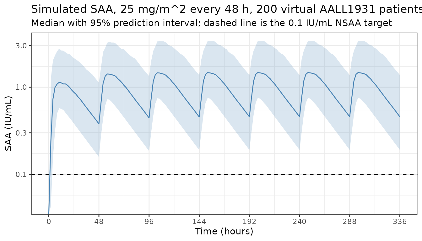
Assumptions and deviations / Errata
The model’s amount unit is IU, and no mg-to-IU conversion is published. The zero-order absorption rate is reported in IU/h in both Lin 2023 Table 2 and Lin 2021 Table 2, and
Cc = central / vcis IU/mL only if the dose is in IU. Neither publication states the specific activity of JZP458, so a 25 mg/m^2 dose cannot be expressed in model units from any published source. Dose this model in IU. No conversion factor is present in the model file.The dose scale used below the “Dose-scale reconstruction” heading is figure-derived, not published. It is obtained by calibrating the model to one landmark digitised from Lin 2023 Figure 3b (the first peak of the 25 mg/m^2 every-48-h median profile, about 1.0 IU/mL), which implies roughly 580 IU/mg. That calibration then reproduces three landmarks it was not fitted to – the steady-state peak and trough of the same figure, and the order of magnitude of the Results-text Tmax – which is the only evidence offered for it. Because it is a single eyeball read off a log axis, it is good to about one significant figure and is used only for illustration; it is flagged inline wherever it is used and appears nowhere in the model file.
Absorption structure was inferred from prose plus the parameter set, not from a printed equation. Lin 2023 prints the two covariate equations but no absorption equation. The encoding here – a zero-order input filling the depot at
R1while first-orderKadrains it – is the reading that (a) matches “zero-order infusion followed by a first-order absorption”, (b) uses exactly the three reported fixed parametersKa,R1andF, (c) matches NONMEM’s reservedR1rate-for-compartment-1 semantics, and (d) is the only reading that reproduces the published terminal half-life. A parallel zero-plus-first-order absorption out of the depot was rejected because the depot then empties in finite time and the terminal half-life collapses tolog(2)/kel = 2.1 hinstead of the reported 19.1 h.Median Tmax is only approximately reproduced, and only under the reconstructed dose scale. Lin 2023 reports a median individual predicted Tmax of 12.0 h with a range of 4-24 h. The value the model gives at the reconstructed scale is printed in the held-out-landmarks table above and sits inside that range. Tmax scales with the dose through the zero-order input duration
F * amt / R1, so it is not a dose-independent check and it cannot be used to arbitrate the scale. Note also that every reported Tmax value (median 12.0, range 4 and 24) is a multiple of 4 h, which suggests the post-hoc Tmax was read off a 4-hourly output grid rather than a continuous optimum.Table 2 labels the bioavailability row “(%)” but the value is a fraction.
F = 0.359is 35.9%, not 0.359%. Two checks in the upstream Lin 2021 settle it: its Table 2 givesF = 0.365while its Results text calls the same quantity “bioavailability at 36.5%”, and its Table 2 footnote reconcilesVd = 3030 mL(i.v.) againstVd/F = 8.30 L(i.m.), which requires3030 / 0.365 = 8301 mL. Taking the header literally would inflate the apparent volume a hundredfold, so the fraction reading is encoded.$SIGMAfixed to 1 is not a third error term. Lin 2023 Table 2’s final row, “Within-subject variability | Proportional | 1 | 100%”, is the NONMEM idiom of fixing$SIGMAto 1 so the residual magnitudes are carried by the two$THETArows above it. It is encoded here aspropSd = 0.46andaddSd = 0.0166with no additional parameter.No CL-V correlation is encoded. Lin 2023 reports IIV on clearance and volume separately and no covariance, so the two etas are left uncorrelated.
T-ALL is not T-lineage. The retained covariate is the T-cell ALL subtype only. The 9.6% of patients with T-cell lymphoblastic lymphoma are in the reference group, because Lin 2023 screened primary disease (ALL vs LBL) and disease subtype (B vs T cell) as separate covariates and retained only the T-ALL cell of that cross-classification.
Table 1 misprints the age range. Lin 2023 Table 1 gives age as “10.0 (1.7-2.5)”, which contradicts both the same table’s mean of 10.2 years and the Results text, “ranged from 1.7 to 25 years of age”. The model’s
populationmetadata records the text value, 1.7-25 years.Screened-but-not-retained covariates are documented, not modelled. Age, sex, height, body weight, ethnicity, primary disease and ADA status were all evaluated and rejected. They are recorded in the model file’s
covariatesDataExcludedlist so the composition of the covariate screen is auditable without introducing unusedcovariateDataentries.The virtual cohort is illustrative. Lin 2023’s published response rates were computed on a 2000-subject NHANES virtual population constructed to match real-world ALL race epidemiology. The 200-subject cohort here matches the AALL1931 analysis-set covariate distributions instead, and additionally depends on the reconstructed dose scale, so its response rate is not a like-for-like reproduction of the published 93.8%.