Eltrombopag (Farrell 2014)
Source:vignettes/articles/Farrell_2014_eltrombopag.Rmd
Farrell_2014_eltrombopag.RmdModel and source
- Citation: Farrell C, Hayes S, Wire M, Zhang J. Population pharmacokinetic/pharmacodynamic modelling of eltrombopag in healthy volunteers and subjects with chronic liver disease. Br J Clin Pharmacol. 2014 May;77(5):717-728. doi:10.1111/bcp.12244.
- Description: Population PK/PD model for eltrombopag in healthy male volunteers (single dose) and adult patients with chronic liver disease (CLD; multiple daily doses) (Farrell 2014). Two-compartment apparent disposition with dual sequential first-order absorption: Ka1 acts on the depot from the end of the absorption lag time (ALAG1) until time MTIME after the dose, and Ka2 acts thereafter. CL/F is reduced in females, in East Asian subjects, and in CLD patients with a linear-in-Child-Pugh-score gradient (HEPIMP_CP_SCORE >= 5). Vc/F is approximately three-fold higher in South/Central Asian subjects. Platelet dynamics use a four-compartment lifespan model (three maturing precursor pools feeding the circulating-platelet pool) with linear stimulation of precursor production by plasma eltrombopag; the slope SLOP is 34% lower in East Asian CLD patients. PD parameters are CLD-specific (median baseline platelet 41 Gi/L).
- Article: https://doi.org/10.1111/bcp.12244
Population
Farrell 2014 pooled data from three studies (Table 1): single oral 30 / 50 / 75 mg eltrombopag in 28 healthy adult male volunteers (Study 1), 12.5 / 25 / 37.5 mg PO QD for 14 days in 38 thrombocytopenic Japanese patients with chronic liver disease (CLD) (Study 2), and 75 mg PO QD for 14 days in 41 CLD patients of mixed race (Study 3). The population PK data set covers 786 plasma concentrations from all 107 subjects; the population PK/PD data set covers 451 platelet count observations from the 79 CLD patients only.
Median (range) age was 50 (19-81) years and median body weight 67.9 (40.6-102) kg; 27% of subjects were female. The race distribution (Table 2) was 35% White, 2% Black / African-American, 42% East Asian (38 Japanese CLD patients in Study 2 plus 7 East Asian patients in Study 3), 20% South / Central Asian, and 2% “Other”. Among the 79 CLD patients, 37 were Child-Pugh Class A (score 5-6), 40 Class B (score 7-9), and 2 Class C (score 10-15); the median (range) baseline platelet count was 41 (19-54.5) Gi/L.
The same fields are available programmatically as
readModelDb("Farrell_2014_eltrombopag")$population.
Source trace
Per-parameter origin is recorded inline next to each
ini() entry in
inst/modeldb/specificDrugs/Farrell_2014_eltrombopag.R. The
table below collects them in one place.
| Equation / parameter | Value | Source location |
|---|---|---|
lcl (CL/F, L/h) |
0.953 | Farrell 2014 Table 3 (NONMEM point estimate, reference White male HV) |
lvc (Vc/F, L) |
9.75 | Farrell 2014 Table 3 (non-S/C-Asian reference) |
lvp (Vp/F, L) |
9.41 | Farrell 2014 Table 3 |
lq (Q/F, L/h) |
0.633 | Farrell 2014 Table 3 |
lka1 (Ka1, 1/h, pre-MTIME) |
0.333 | Farrell 2014 Table 3 |
lka2 (Ka2, 1/h, post-MTIME) |
5.26 | Farrell 2014 Table 3 |
ltlag (ALAG1, h) |
0.447 | Farrell 2014 Table 3 |
ltswitch (paper MTIME, h) |
1.46 | Farrell 2014 Table 3 (renamed: rxode2 reserves
mtime) |
e_sexf_cl |
-0.378 | Farrell 2014 Table 3, ‘CL/F ~ Females’ multiplier 0.622 |
e_neas_cl |
-0.524 | Farrell 2014 Table 3, ‘CL/F ~ East Asians’ multiplier 0.476 |
e_cp_cl (CP-anchor) |
0.536 | Farrell 2014 Table 3, ‘CL/F ~ CP Score 5’ |
e_cp_slope (per-unit decr.) |
-0.113 | Farrell 2014 Table 3 footnote, ‘CL/F ~ CP Score > 5’ |
e_scasian_vc |
1.98 | Farrell 2014 Table 3, ‘Vc/F ~ South/Central Asians’ multiplier 2.98 |
| PK IIV block CL-Vc | (0.161, 0.106, 0.233) | Farrell 2014 Table 3 (CV 40%, 48%, R=0.547) |
| PK IIV Ka1 (paper: IOV) | 1.61 | Farrell 2014 Table 3 omega^2_Ka |
propSd (Cc) |
0.154 | Farrell 2014 Table 3 sqrt(sigma^2_prop = 0.0237) |
addSd (Cc, ug/mL) |
0.0333 | Farrell 2014 Table 3 sqrt(sigma^2_add = 1110 ng2/mL2) / 1000 |
lslop (mL/ug) |
0.648 | Farrell 2014 Table 6 |
lkin (Gi/L/h) |
0.211 | Farrell 2014 Table 6 |
lkt (1/h) |
0.0214 | Farrell 2014 Table 6 |
lrbase (Gi/L, CLD median) |
41 | Farrell 2014 Table 2 |
e_neas_slop |
-0.340 | Farrell 2014 Table 6, ‘SLOP ~ East Asians’ multiplier 0.660 |
| PD IIV SLOP | 0.287 | Farrell 2014 Table 6 omega^2_SLOP (CV 53.6%) |
| PD IIV KT | 0.313 | Farrell 2014 Table 6 omega^2_KT (CV 55.9%) |
propSd_PLT |
0.444 | Farrell 2014 Table 6 sqrt(sigma^2_prop = 0.197) |
| PK structure: 2-cmt dual ka | - | Farrell 2014 Results ‘Population pharmacokinetic analysis’ paragraph 1 |
| PD structure: 4-cmt lifespan | - | Farrell 2014 Results ‘Population pharmacokinetic/pharmacodynamic analysis’ |
Virtual cohort
The vignette uses five typical-value subgroups, each set up as a single representative subject (one ID per subgroup). Etas are zeroed so each profile is the population median for the named covariate combination. CP score 5 stands in for “Child-Pugh Class A” (lowest score in the class); CP score 7 stands in for “Class B”; healthy volunteers carry CP score 0 to gate the CP effect off.
set.seed(20140414)

# Each scenario row gives one subject with a deterministic covariate vector.
scenarios <- tibble::tribble(
  ~treatment,                            ~SEXF, ~RACE_ASIAN_NORTHEAST, ~RACE_ASIAN_SOUTHCENTRAL, ~HEPIMP_CP_SCORE,
  "HV reference (White male, healthy)",   0,     0,          0,                        0,
  "CLD non-EA male, Class A (CP=5)",      0,     0,          0,                        5,
  "CLD non-EA female, Class A (CP=5)",    1,     0,          0,                        5,
  "CLD East Asian male, Class A (CP=5)",  0,     1,          0,                        5,
  "CLD non-EA male, Class B (CP=7)",      0,     0,          0,                        7
) |>
  dplyr::mutate(id = dplyr::row_number())

# 50 mg PO QD x 14 days; PKNCA analyses the last dosing interval (steady state).
tau    <- 24
n_dose <- 14
dose_times <- seq(0, by = tau, length.out = n_dose)
pk_obs_times <- sort(unique(c(
  seq(0.001, tau,                  by = 0.25),                # dense first day (avoid t = 0 collision with dose)
  seq(0,     n_dose * tau,         by = 2),                   # daily window across the regimen
  (n_dose - 1) * tau + seq(0, tau, by = 0.25)                 # dense final dosing interval
)))
# PD observations through the regimen plus 14-day off-treatment recovery window.
pd_obs_times <- sort(unique(seq(0, n_dose * tau + 14 * 24, by = 12)))

dose_rows <- scenarios |>
  tidyr::expand_grid(time = dose_times) |>
  dplyr::mutate(evid = 1L, amt = 50, cmt = "depot")

pk_obs_rows <- scenarios |>
  tidyr::expand_grid(time = pk_obs_times) |>
  dplyr::mutate(evid = 0L, amt = NA_real_, cmt = "Cc")

pd_obs_rows <- scenarios |>
  tidyr::expand_grid(time = pd_obs_times) |>
  dplyr::mutate(evid = 0L, amt = NA_real_, cmt = "PLT")

events <- dplyr::bind_rows(dose_rows, pk_obs_rows, pd_obs_rows) |>
  dplyr::arrange(id, time, dplyr::desc(evid)) |>
  dplyr::select(id, time, evid, amt, cmt,
                treatment, SEXF, RACE_ASIAN_NORTHEAST,
                RACE_ASIAN_SOUTHCENTRAL, HEPIMP_CP_SCORE)

stopifnot(!anyDuplicated(unique(events[, c("id", "time", "evid", "cmt")])))
Simulation
mod_typical <- rxode2::zeroRe(mod_fun)   # typical-value (median) simulation
#> ℹ parameter labels from comments will be replaced by 'label()'

sim <- rxode2::rxSolve(
  mod_typical,
  events = events,
  keep   = c("treatment", "SEXF", "RACE_ASIAN_NORTHEAST",
             "RACE_ASIAN_SOUTHCENTRAL", "HEPIMP_CP_SCORE",
             "cmt"),
  returnType = "data.frame"
)
#> ℹ omega/sigma items treated as zero: 'etalcl', 'etalvc', 'etalka1', 'etalslop', 'etalkt'
#> Warning: multi-subject simulation without without 'omega'

# Tag each output row by the observable it carries; PK observations land on the
# `Cc`-tagged rows from `events`, PD observations on the `PLT`-tagged rows.
sim_pk <- sim |> dplyr::filter(cmt == "Cc",  !is.na(Cc))
sim_pd <- sim |> dplyr::filter(cmt == "PLT", !is.na(PLT))
The simulation returns one row per subject x time x evid;
Cc is in ug/mL and PLT in Gi/L.
Replicate published figures
Plasma eltrombopag concentration over the final dosing interval
sim_pk |>
  dplyr::filter(time >= (n_dose - 1) * tau,
                time <= n_dose * tau) |>
  dplyr::mutate(time_in_tau = time - (n_dose - 1) * tau) |>
  ggplot(aes(time_in_tau, Cc, colour = treatment)) +
  geom_line() +
  scale_x_continuous("Time after final dose (h)", breaks = seq(0, 24, 4)) +
  scale_y_continuous("Plasma eltrombopag Cc (ug/mL)") +
  labs(colour = NULL,
       title = "Typical-value steady-state Cc (50 mg PO QD x 14 d)") +
  theme(legend.position = "bottom") +
  guides(colour = guide_legend(nrow = 3))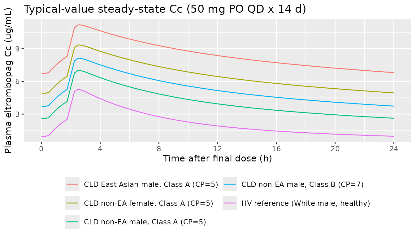
Steady-state Cc over the last dosing interval (24 h after dose 14), 50 mg eltrombopag PO QD for 14 days. Replicates the right-hand panel of Figure 2 (prediction-corrected VPC for CLD steady-state) for the median trajectories; the original figure overlays observed CLD data which are not available outside the study database.
Platelet count response over the full regimen
The platelet panel applies only to CLD subjects (the source PD model was fit on CLD data); the HV row is shown for reference because the typical-value healthy CL/F drives lower exposures and therefore much less stimulation.
sim_pd |>
  ggplot(aes(time / 24, PLT, colour = treatment)) +
  geom_line() +
  geom_vline(xintercept = n_dose, linetype = "dashed", colour = "grey50") +
  annotate("text", x = n_dose, y = Inf, label = " end of dosing",
           hjust = 0, vjust = 1.5, size = 3, colour = "grey40") +
  scale_x_continuous("Time (days)") +
  scale_y_continuous("Platelet count (Gi/L)") +
  labs(colour = NULL,
       title = "Typical-value platelet response by subgroup") +
  theme(legend.position = "bottom") +
  guides(colour = guide_legend(nrow = 3))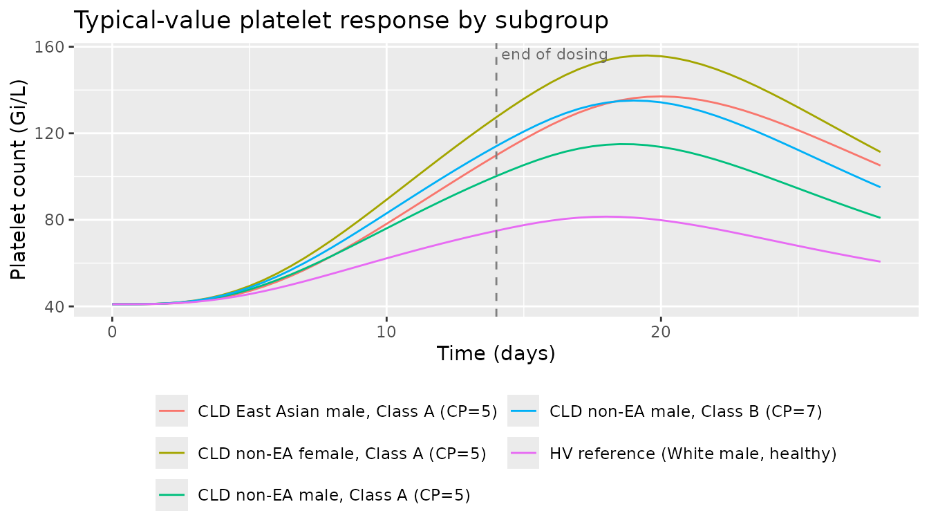
Typical-value platelet response across the 14-day regimen and the 14-day off-treatment recovery window, by CLD covariate subgroup. Replicates the CLD trace of Figure 6 (cross-population time course at 50 mg PO QD x 14 d), without the HCV / ITP / HV reference traces. PD parameters are CLD-calibrated; the HV row is included only to show the qualitative reduction in drug-driven stimulation.
PKNCA validation
NCA at steady state (final dosing interval) for each subgroup.
Cmax,ss and AUC0-tau are compared against Farrell 2014 Table 4
(dose-normalised to 50 mg QD); the model file’s units
metadata sets the unit declarations passed to PKNCA.
sim_nca_input <- sim_pk |>
  dplyr::filter(time >= (n_dose - 1) * tau,
                time <= n_dose * tau) |>
  dplyr::select(id, time, Cc, treatment)

# Defensive: PKNCA's auclast on a [start, end] interval needs a row at `start`.
# Add a row at start with the simulated Cc at the start time if not already there.
sim_nca_input <- sim_nca_input |>
  dplyr::distinct(id, treatment, time, .keep_all = TRUE) |>
  dplyr::arrange(id, treatment, time)

dose_df <- events |>
  dplyr::filter(evid == 1) |>
  dplyr::select(id, time, amt, treatment)

conc_obj <- PKNCA::PKNCAconc(sim_nca_input,
                             Cc ~ time | treatment + id,
                             concu = "ug/mL", timeu = "h")
dose_obj <- PKNCA::PKNCAdose(dose_df,
                             amt ~ time | treatment + id,
                             doseu = "mg")

start_ss <- (n_dose - 1) * tau
end_ss   <- n_dose * tau

intervals <- data.frame(
  start    = start_ss,
  end      = end_ss,
  cmax     = TRUE,
  tmax     = TRUE,
  auclast  = TRUE,
  cav      = TRUE,
  half.life = TRUE
)

nca_res <- PKNCA::pk.nca(PKNCA::PKNCAdata(conc_obj, dose_obj,
                                          intervals = intervals))
Comparison against Farrell 2014 Table 4
Farrell 2014 Table 4 reports geometric-mean (95% CI) post-hoc estimates of CL/F, t1/2, AUC(0-tau), and Cmax at 50 mg eltrombopag QD steady state for several CLD subgroups. Each row of the comparison below selects the single typical-value subject whose covariate vector matches the subgroup most directly. Differences > 20% reflect the fact that Table 4 averages over the actual covariate distribution inside each subgroup (e.g. “CLD Males” includes a mix of races and Child-Pugh classes); the typical-value row uses one fixed covariate vector per scenario.
published <- tibble::tribble(
  ~treatment,                              ~cmax,  ~auclast, ~half.life,
  "HV reference (White male, healthy)",     5.37,    53.0,    21.1,
  "CLD non-EA male, Class A (CP=5)",       10.8,   156.0,    70.5,
  "CLD non-EA female, Class A (CP=5)",     19.2,   285.0,    92.3,
  "CLD East Asian male, Class A (CP=5)",   19.7,   287.0,    81.2,
  "CLD non-EA male, Class B (CP=7)",       15.5,   234.0,    86.3
)

cmp <- nlmixr2lib::ncaComparisonTable(
  simulated = nca_res,
  reference = published,
  by        = "treatment",
  units     = c(cmax = "ug/mL", auclast = "ug*h/mL",
                tmax = "h",    half.life = "h"),
  tolerance_pct = 20
)

knitr::kable(
  cmp,
  caption = paste(
    "Simulated typical-value steady-state NCA (50 mg PO QD x 14 d) vs.",
    "Farrell 2014 Table 4 dose-normalised geometric means.",
    "* differs from reference by >20%; see Assumptions and deviations for context."
  ),
  align = c("l", "l", "r", "r", "r")
)| NCA parameter | treatment | Reference | Simulated | % diff |
|---|---|---|---|---|
| Cmax (ug/mL) | HV reference (White male, healthy) | 5.37 | 5.27 | -1.8% |
| Cmax (ug/mL) | CLD non-EA male, Class A (CP=5) | 10.8 | 7.01 | -35.1%* |
| Cmax (ug/mL) | CLD non-EA female, Class A (CP=5) | 19.2 | 9.35 | -51.3%* |
| Cmax (ug/mL) | CLD East Asian male, Class A (CP=5) | 19.7 | 11.2 | -43.2%* |
| Cmax (ug/mL) | CLD non-EA male, Class B (CP=7) | 15.5 | 8.14 | -47.5%* |
| AUClast (ug*h/mL) | HV reference (White male, healthy) | 53 | 52.5 | -0.9% |
| AUClast (ug*h/mL) | CLD non-EA male, Class A (CP=5) | 156 | 97.9 | -37.3%* |
| AUClast (ug*h/mL) | CLD non-EA female, Class A (CP=5) | 285 | 156 | -45.1%* |
| AUClast (ug*h/mL) | CLD East Asian male, Class A (CP=5) | 287 | 202 | -29.7%* |
| AUClast (ug*h/mL) | CLD non-EA male, Class B (CP=7) | 234 | 126 | -46.1%* |
| t½ (h) | HV reference (White male, healthy) | 21.1 | 15.9 | -24.5%* |
| t½ (h) | CLD non-EA male, Class A (CP=5) | 70.5 | 25.1 | -64.3%* |
| t½ (h) | CLD non-EA female, Class A (CP=5) | 92.3 | 37.9 | -58.9%* |
| t½ (h) | CLD East Asian male, Class A (CP=5) | 81.2 | 48.3 | -40.5%* |
| t½ (h) | CLD non-EA male, Class B (CP=7) | 86.3 | 31.2 | -63.9%* |
Assumptions and deviations
Typical-value (median) simulation. All etas are zeroed (
rxode2::zeroRe) so each scenario row is a single representative subject. The paper’s Table 4 reports geometric means across the actual observed covariate distribution inside each subgroup; the vignette compares a single covariate-stratified typical value, so direct equality is not expected. Differences > 20% in the comparison table tag subgroups where the within-subgroup covariate distribution materially differs from the chosen typical vector.Single Child-Pugh score per class. Within the CLD subgroups, this vignette uses the lower bound of each Class (
HEPIMP_CP_SCORE = 5for Class A,= 7for Class B). Subjects with higher scores within a class would have correspondingly lower CL/F per the model’s linear-in-score effect (factor = 0.536 * (1 - 0.113 * (CP - 5))).PK structural simplification: residual-error scaling factors omitted. Farrell 2014 Table 3 reports two factors that scale the proportional residual error for specific sample subsets -
sigma_Prop~HV = 0.453multiplyingpropSdfor healthy-volunteer samples (i.e., healthy-volunteer samples have lower observed-vs-predicted noise) andsigma_Prop~TAD<4h = 1.72multiplyingpropSdfor samples taken within 4 h of dose (early absorption phase, where the dual-Ka switch introduces more model-fit uncertainty). These two factors are simplified out of the registry model, which uses a single proportional+additive error model calibrated to CLD steady-state samples. Vignette VPCs and Table 4 comparisons therefore use the CLD steady-state error parameters throughout.IIV on Ka1 encoded as IIV, paper labelled IOV. Farrell 2014 Table 3 lists
omega^2_Kaunder “Interindividual or interoccasion variability” and the table footnote clarifies it is interoccasion variability (IOV) on Ka1. Because the registry does not carry NONMEM-style occasion structure (no OCC column in the data), the source value is encoded here as IIV on Ka1 (etalka1). Within a single subject this reproduces the magnitude of the per-occasion absorption variability the paper reports, just attributed to the subject rather than to the occasion.Baseline platelet count: typical-value parameter
lrbase, not per-subject covariate. Farrell 2014 derived each subject’s platelet first-order degradation constant KP fromKP = KIN / baseline_PLTusing the observed baseline platelet count, so KP varied across subjects with their actual pre-dose platelet values. The registry model uses the canonical baseline- value parameterlrbaseset to the CLD median 41 Gi/L (Farrell 2014 Table 2) and deriveskdeg = kin / rbasefrom it. Inter-subject baseline-platelet variability is therefore not captured directly; the model’s IIV on KT (etalkt) provides some between-subject variability in the maturation rate and hence in steady-state circulating platelets.PD parameters are CLD-specific. The Farrell 2014 paper notes that the estimated typical KIN (0.211 Gi/L/h) for the CLD population is much lower than the value previously estimated for healthy or ITP populations (1.43); the registry model carries the CLD-specific KIN. Simulating HV subjects with this PD layer therefore produces qualitatively-correct but quantitatively-CLD-scaled platelet responses; do not interpret the HV row of Figure 6 as a quantitative HV prediction.
South/Central Asian Vc/F effect: structural, not pre-validated against Table 4. Table 4 does not stratify by South/Central Asian status, so the comparison table above does not include this subgroup. The Vc/F multiplier 2.98 is taken at face value from Farrell 2014 Table 3 and applied at simulation time when
RACE_ASIAN_SOUTHCENTRAL = 1.Healthy-volunteer doses in Table 4. Study 1 included only single-dose administrations; Table 4 reports dose-normalised steady-state estimates for the HV cohort obtained by repeat-dose extrapolation (Farrell 2014 Results paragraph after Table 3). The vignette simulates 14-day repeat dosing for all scenarios, including HV, so the HV row is consistent with the paper’s extrapolation.
Race-indicator encoding for the East Asian subgroup. In the source data set the East Asian race indicator covers Chinese / Japanese / Korean heritage; all 38 Study 2 patients were Japanese and 7 of Study 3 PK substudy patients were East Asian. The canonical
RACE_ASIAN_NORTHEASTindicator pools these subgroups, matching the source classification.New canonical covariate columns ratified in this PR. Two canonical entries were added to
inst/references/covariate-columns.mdto support this model:RACE_ASIAN_SOUTHCENTRAL(binary indicator analogous toRACE_ASIAN_NORTHEAST) andHEPIMP_CP_SCORE(continuous integer Child-Pugh score, complementing the existing binaryHEPIMP_*family). Naming was ratified by operator response to a Phase 3 sidecar.