Polyclonal immunoglobulin popPK model family (van der Zeeuw 2026)
Source:vignettes/articles/vanderZeeuw_2026_immunoglobulin.Rmd
vanderZeeuw_2026_immunoglobulin.RmdModel and source
This vignette covers twelve population PK models for polyclonal immunoglobulin G (IVIg, SCIg and hyaluronidase-facilitated SCIg), one of which also carries a pharmacodynamic layer. They were extracted together because they come from a single secondary source.
- Article: van der Zeeuw et al., Clinical Pharmacokinetics 2026;65(6):811-36
- Supplement: https://doi.org/10.1007/s40262-026-01641-5 (Supplementary Equations S1-S4)
van der Zeeuw 2026 is a PRISMA systematic review. It develops no model of its own; it catalogues fourteen previously published immunoglobulin popPK(-PD) models and tabulates their structural parameters, inter-individual variability and residual error in its Table 4. Under the standing extract-from-review policy, a review that tabulates the parameters is extracted rather than skipped, with each model file citing both the primary publication and the review as the transcription source.
Everything in these twelve files is a transcription of a secondary source. Each model should be re-verified against its primary publication before being relied on. Per-study re-verification notes are kept in the maintainers’ records.
ig_models <- c(
  # Primary / secondary immunodeficiency
  "Landersdorfer_2013_immunoglobulin",
  "Dumas_2019_immunoglobulin",
  "Tortorici_2019_immunoglobulin",
  "Luo_2020_immunoglobulin",
  "Tegenge_2020_immunoglobulin",
  "Zhang_2020_immunoglobulin",
  "Lee_2021_immunoglobulin",
  "Li_2022_immunoglobulin",
  "NavarroMora_2022_immunoglobulin",
  # Immune-mediated disease
  "Tortorici_2021_immunoglobulin",
  "Li_2024a_immunoglobulin",
  "Li_2024b_immunoglobulin"
)

tibble::tibble(
  Model = ig_models,
  Description = vapply(
    ig_models,
    function(m) rxode2::rxode(readModelDb(m))$description,
    character(1)
  )
) |>
  knitr::kable()
#> ℹ parameter labels from comments will be replaced by 'label()'
#> ℹ parameter labels from comments will be replaced by 'label()'
#> ℹ parameter labels from comments will be replaced by 'label()'
#> ℹ parameter labels from comments will be replaced by 'label()'
#> ℹ parameter labels from comments will be replaced by 'label()'
#> ℹ parameter labels from comments will be replaced by 'label()'
#> ℹ parameter labels from comments will be replaced by 'label()'
#> ℹ parameter labels from comments will be replaced by 'label()'
#> ℹ parameter labels from comments will be replaced by 'label()'
#> ℹ parameter labels from comments will be replaced by 'label()'
#> ℹ parameter labels from comments will be replaced by 'label()'| Model | Description |
|---|---|
| Landersdorfer_2013_immunoglobulin | Two-compartment population PK model with first-order subcutaneous absorption for polyclonal immunoglobulin G (IVIg and SCIg) in primary immunodeficiency (Landersdorfer 2013) |
| Dumas_2019_immunoglobulin | One-compartment population PK model with first-order subcutaneous absorption for polyclonal immunoglobulin G (IVIg and SCIg 20%, Ig20Gly) in primary immunodeficiency (Dumas 2019) |
| Tortorici_2019_immunoglobulin | Two-compartment population PK model for intravenous polyclonal immunoglobulin G (Privigen) in primary and secondary immunodeficiency, with a disease-type effect on central volume (Tortorici 2019) |
| Luo_2020_immunoglobulin | Two-compartment population PK model with first-order subcutaneous absorption for polyclonal immunoglobulin G (IgPro10) in Japanese and non-Japanese patients with primary immunodeficiency (Luo 2020) |
| Tegenge_2020_immunoglobulin | Two-compartment population PK model for intravenous polyclonal immunoglobulin G in very low birth-weight neonates (Tegenge 2020) |
| Zhang_2020_immunoglobulin | Two-compartment population PK model with first-order subcutaneous absorption for polyclonal immunoglobulin G (IgPro20, Hizentra) given weekly or biweekly in primary immunodeficiency (Zhang 2020) |
| Lee_2021_immunoglobulin | One-compartment population PK model for intravenous polyclonal immunoglobulin G in patients with predominantly antibody deficiencies, fitted to endogenous-subtracted (exogenous) IgG concentrations (Lee 2021) |
| Li_2022_immunoglobulin | Two-compartment population PK model with first-order subcutaneous absorption for polyclonal immunoglobulin G across intravenous, subcutaneous and hyaluronidase-facilitated subcutaneous products in primary immunodeficiency, scaled on lean body mass (Li 2022) |
| NavarroMora_2022_immunoglobulin | Two-compartment population PK model with first-order subcutaneous absorption for polyclonal immunoglobulin G given subcutaneously or intravenously in primary immunodeficiency (Navarro-Mora 2022) |
| Tortorici_2021_immunoglobulin | Two-compartment population PK model with first-order subcutaneous absorption for polyclonal immunoglobulin G in chronic inflammatory demyelinating polyneuropathy (Tortorici 2021) |
| Li_2024a_immunoglobulin | One-compartment population PK model for intravenous polyclonal immunoglobulin G in multifocal motor neuropathy, scaled on lean body mass (Li 2024, Frontiers in Neurology) |
| Li_2024b_immunoglobulin | One-compartment population PK model with a grip-strength indirect-response pharmacodynamic layer for intravenous polyclonal immunoglobulin G in multifocal motor neuropathy (Li 2024, Annals of Clinical and Translational Neurology) |
Population
The twelve cohorts span the full clinical range over which immunoglobulin is given. Nine are immunoglobulin replacement therapy in primary (and in one case secondary) immunodeficiency, where doses are low and the therapeutic goal is to restore a physiological IgG concentration. Three are immunomodulatory therapy in immune-mediated neuropathy (CIDP, MMN), where doses are roughly five times higher and the goal is an anti-inflammatory effect.
Cohort sizes run from 10 (Lee 2021, a Malaysian cohort of predominantly X-linked agammaglobulinaemia patients) to 340 (Li 2022, pooling eight trials). Reference weights run from 27 kg (Lee 2021) to 82 kg (Tortorici 2021), and Tegenge 2020 sits apart entirely: very low birth-weight preterm neonates with birth weights of 0.78-1.38 kg. All adult/paediatric cohorts pooled children and adults, and age was not retained as a covariate in any of the fourteen reviewed models (van der Zeeuw 2026 section 3.2.1.5); body weight, through allometric scaling, does the work instead.
Full per-cohort demographics are available programmatically:
pop_row <- function(m) {
  p <- readModelDb(m)()$population
  tibble::tibble(
    Model      = m,
    N          = p$n_subjects,
    `Age`      = p$age_range %||% NA_character_,
    `Weight`   = p$weight_range %||% NA_character_,
    `Indication` = p$disease_state
  )
}
`%||%` <- function(a, b) if (is.null(a)) b else a

purrr_free <- do.call(rbind, lapply(ig_models, pop_row))
knitr::kable(purrr_free)| Model | N | Age | Weight | Indication |
|---|---|---|---|---|
| Landersdorfer_2013_immunoglobulin | 151 | 3-81 years (per-study medians 18.0-32.0 years) | 13.0-135.0 kg (per-study medians 53.5-66.5 kg) | Primary immunodeficiency (PID) on immunoglobulin replacement therapy |
| Dumas_2019_immunoglobulin | 102 | 2.0-83 years | 13.2-161.8 kg | Primary immunodeficiency (PID) on immunoglobulin replacement therapy |
| Tortorici_2019_immunoglobulin | 187 | PID mean (SD) 29.8 (20.3) years; SID mean (SD) 69.5 (10.4) years | PID mean (SD) 62.6 (26.4) kg; SID mean (SD) 76.8 (16.1) kg | Primary immunodeficiency (PID, n = 90) and secondary immunodeficiency (SID, n = 97) |
| Luo_2020_immunoglobulin | 202 | 3-81 years | 13-135 kg | Primary immunodeficiency (PID) on immunoglobulin replacement therapy |
| Tegenge_2020_immunoglobulin | 20 | 1-6 days postnatal | 0.78-1.38 kg (birth weight) | Very low birth-weight preterm neonates receiving intravenous immunoglobulin |
| Zhang_2020_immunoglobulin | 173 | 3.0-81.0 years (per-study medians 18.0-32.0 years) | 13.0-135.0 kg | Primary immunodeficiency (PID) on immunoglobulin replacement therapy |
| Lee_2021_immunoglobulin | 10 | 3-64 years | 9.3-75 kg | Predominantly antibody deficiency (a form of primary immunodeficiency); the cohort was mainly X-linked agammaglobulinaemia (XLA) patients |
| Li_2022_immunoglobulin | 340 | 2.0-83.0 years | 11.9-162 kg | Primary immunodeficiency (PID) on immunoglobulin replacement therapy |
| NavarroMora_2022_immunoglobulin | 95 | Not reported as a range; per-study means 10.8-42.5 years | 16.7-153.0 kg | Primary immunodeficiency (PID) on immunoglobulin replacement therapy |
| Tortorici_2021_immunoglobulin | 235 | 22-83 years | 42.3-133 kg | Chronic inflammatory demyelinating polyneuropathy (CIDP) |
| Li_2024a_immunoglobulin | 44 | 31.0-72.0 years | 56.3-107.0 kg | Multifocal motor neuropathy (MMN) |
| Li_2024b_immunoglobulin | 44 | 31.0-72.0 years | 56.3-107.0 kg | Multifocal motor neuropathy (MMN) |
Source trace
Every ini() entry in every one of the twelve model files
carries a trailing comment naming its source location. The table below
collects the structural fixed effects in one place. BW is
body weight and LBM lean body mass, each divided by the
reference value printed in the source.
| Model | CL or Kel (/day or L/day) | Vc (L) | Q (L/day) | Vp (L) | F1 (SC) | Ka (/day) | Source |
|---|---|---|---|---|---|---|---|
| Landersdorfer 2013 | 0.142 | 3.94 | 0.252 | 4.18 | 66.0% | 0.439 | Table 4 |
| Dumas 2019 | 0.09216*(BW/70)^0.576 | 4.01 | - | - | 73.9% | 0.096 | Table 4 |
| Tortorici 2019 | 0.152*(BW/72)^0.796 | 3.08*(BW/72)^1.1 (PID); 8.75 (SID) | 0.825 | 1.8 | - | - | Table 4 |
| Luo 2020 | 0.139*(BW/58.7)^0.881 | 4.01*(BW/58.7)^0.501 | 0.300 | 3.51 | 66.8% | 0.506 | Table 4 |
| Tegenge 2020 | 0.0027 | 0.008 | 0.045 | 0.055 | - | - | Table 4 |
| Zhang 2020 | 0.138*(BW/66)^0.768 | 3.95*(BW/66)^0.448 | 0.260 | 4.44 | 67.6% | 0.444 | Table 4 |
| Lee 2021 | 0.0624*(BW/27)^0.88 | 2.77*(BW/27)^0.66 | - | - | - | - | Table 4 |
| Li 2022 | 0.183*(LBM/47)^0.75 | 3.01*(LBM/47)^1 | 0.353*(LBM/47)^0.75 | 1.40*(LBM/47)^1 | 70.5% / 79.4% (fSCIg) | 0.395 | Table 4 |
| Navarro-Mora 2022 | 0.150*(BW/65.7)^0.744 | 3.06*(BW/65.7)^0.686 | 0.474 | 1.93*(BW/65.7)^1.04 | 70.5% | 0.246 | Table 4 |
| Tortorici 2021 | 0.435*(BW/82)^0.615 | 4.69*(BW/82)^0.773 | 0.50*(BW/82)^0.615 | 1.87*(BW/82)^0.773 | 82.4% | 0.439 (fixed) | Table 4; section 3.2.2.2 |
| Li 2024a (Front Neurol) | Kel = 0.05784 | 6.59*(LBM/56.54)^2.23 | - | - | - | - | Table 4 |
| Li 2024b (Ann Clin Transl Neurol) | Kel = 0.05832 | 6.48*(LBM/56.54)^2.17 | - | - | - | - | Table 4 |
Endogenous IgG and the random-effects structure are traced per model
in the ini() comments. Two conventions apply uniformly and
are stated by the review itself:
-
Inter-individual variability. van der Zeeuw 2026
section 2.3 harmonised every reported IIV to an apparent CV%, so each
file converts back with
omega^2 = log(1 + CV^2). This is a genuine advantage of this review over a typical secondary source, which usually reproduces each primary’s own convention unharmonised. -
Residual error. Table 4 mixes three notations, and
they are read literally: a bare percentage is a proportional SD;
sigma^2 = vis a variance, entered assqrt(v); a bare value in theAdd (g/L)column is an additive SD in g/L. The review distinguishessigmafromsigma^2within the same table (Fokkink 2022 is printed assigma = 0.12), which is what licenses taking the squared notation at face value.
The pharmacodynamic layer of Li 2024b comes from section 3.3.1 and Supplementary Equations S1-S2:
| PD parameter | Value | Source |
|---|---|---|
lrbase (G_BASE, baseline grip strength) |
10.6 kg (IIV 86.8% CV) | section 3.3.1 |
lkout (DTR, deterioration rate) |
0.023 /h = 0.552 /day | section 3.3.1 |
lec50 (C50) |
9.41 g/L | section 3.3.1 |
imax |
0.6066, from LIMAX = 0.433 | section 3.3.1; Eq. S2 |
propSd_gs |
0.0602 | section 3.3.1 |
Virtual cohort
The review’s own cross-model comparison (its Figure 2) uses a single standardised typical patient, which is what makes the twelve models commensurable. Reproducing it requires no stochastic cohort at all: one typical-value profile per model.
van der Zeeuw 2026 section 2.4 specifies the patient as male, 70 kg, 170 cm, with lean body mass from the Boer formula.
# Boer formula for men: LBM = 0.407*WT + 0.267*HT - 19.2 (van der Zeeuw 2026
# section 2.3, citing reference 32).
wt_kg <- 70
ht_cm <- 170
lbm_kg <- 0.407 * wt_kg + 0.267 * ht_cm - 19.2
lbm_kg
#> [1] 54.68
Section 2.4 also fixes the endogenous IgG used for the comparison, overriding whatever each individual model assumed: 4.0 g/L for PID and 10 g/L for CIDP, MMN and GBS. Applying that override is essential – without it the panel would be comparing baselines rather than dispositions.
indication <- c(
  Landersdorfer_2013_immunoglobulin = "PID",
  Dumas_2019_immunoglobulin         = "PID",
  Tortorici_2019_immunoglobulin     = "PID",
  Luo_2020_immunoglobulin           = "PID",
  Tegenge_2020_immunoglobulin       = "neonatal",
  Zhang_2020_immunoglobulin         = "PID",
  Lee_2021_immunoglobulin           = "PID",
  Li_2022_immunoglobulin            = "PID",
  NavarroMora_2022_immunoglobulin   = "PID",
  Tortorici_2021_immunoglobulin     = "CIDP/MMN",
  Li_2024a_immunoglobulin           = "CIDP/MMN",
  Li_2024b_immunoglobulin           = "CIDP/MMN"
)

# Which models carry subcutaneous (depot) data, i.e. reported an F1 and a Ka.
has_sc <- c(
  "Landersdorfer_2013_immunoglobulin", "Dumas_2019_immunoglobulin",
  "Luo_2020_immunoglobulin", "Zhang_2020_immunoglobulin",
  "Li_2022_immunoglobulin", "NavarroMora_2022_immunoglobulin",
  "Tortorici_2021_immunoglobulin"
)

endogenous_igg <- c(PID = 4.0, `CIDP/MMN` = 10.0, neonatal = 5.0)
Tegenge 2020 is carried through the machinery below but excluded from the Figure 2 panels, exactly as the review excludes it (section 3.2.3): it is a neonatal model and a 70 kg dose is meaningless for it.
Simulation
# Solve one model at typical values (no IIV) for a given event table.
# `omega = NA` is NOT used: it fails on models that declare no eta at all
# (Landersdorfer 2013 is one), so zeroRe() is applied conditionally instead.
solve_typical <- function(model_name, ev_dose, times, bl_override) {
  mod <- rxode2::rxode(readModelDb(model_name))
  # Override the endogenous IgG with the review's standardised assumption.
  mod <- do.call(rxode2::ini, list(mod, bl_igg = bl_override))
  if (any(!is.na(mod$iniDf$neta1))) {
    mod <- rxode2::zeroRe(mod)
  }
  # Sampling records: eleven of the twelve models declare a SINGLE endpoint, so
  # a bare time grid is unambiguous and rxSolve returns every model variable as
  # a column. Li 2024b declares TWO endpoints (`Cc` and `gs`); rxode2 then
  # requires each observation row to name which ENDPOINT it belongs to, so the
  # grid is tagged with `cmt = "Cc"` there. That is endpoint naming, not the
  # `cmt = "<observable>"` antipattern: `Cc` is a declared endpoint of every one
  # of these models, so no `cmt()` slot is auto-injected and no ODE state is
  # renumbered. Both `central` and `gs` still come back as columns.
  ev <- if (nrow(mod$predDf) > 1) {
    rxode2::et(ev_dose, times, cmt = "Cc")
  } else {
    rxode2::et(ev_dose, times)
  }
  out <- rxode2::rxSolve(
    mod, ev,
    params = c(WT = wt_kg, LBM = lbm_kg, DIS_SAD = 0, FORM_IG_HYALURONIDASE = 0),
    returnType = "data.frame"
  )
  out$model <- model_name
  out
}
Figure 2A: intravenous immunoglobulin
Dosing per van der Zeeuw 2026 section 2.4. PID: 400 mg/kg loading, then 400 mg/kg once every four weeks. CIDP and MMN: 2000 mg/kg split over five days as a loading dose, then 1000 mg/kg once every three weeks.
n_cycles <- 18  # long enough to reach steady state for a ~40 day half-life

# Dosing records name the ODE state they enter. Sampling times are kept
# SEPARATE and attached inside solve_typical(), which tags them per model
# according to how many endpoints that model declares.
ev_iv_pid <-
  rxode2::et(amt = 0.400 * wt_kg, cmt = "central", ii = 28, addl = n_cycles)
t_iv_pid <- seq(0, 28 * (n_cycles + 1), by = 0.5)

# 2000 mg/kg over five days = five daily 400 mg/kg infusions, then 1000 mg/kg Q3W
ev_iv_imm <-
  rxode2::et(amt = 0.400 * wt_kg, cmt = "central", ii = 1, addl = 4) |>
  rxode2::et(amt = 1.000 * wt_kg, cmt = "central", time = 21, ii = 21,
             addl = n_cycles)
t_iv_imm <- seq(0, 21 * (n_cycles + 2), by = 0.5)
fig2a_models <- setdiff(ig_models, "Tegenge_2020_immunoglobulin")

# Models expose different internal variables (only Li 2024b has `gs`, only the
# two-compartment models have `vp`), so keep the common columns before binding.
common_cols <- function(d) d[, c("time", "Cc", "model")]

sim_iv <- do.call(rbind, lapply(fig2a_models, function(m) {
  ind <- indication[[m]]
  common_cols(
    if (ind == "PID") {
      solve_typical(m, ev_iv_pid, t_iv_pid, endogenous_igg[[ind]])
    } else {
      solve_typical(m, ev_iv_imm, t_iv_imm, endogenous_igg[[ind]])
    }
  )
}))
#> ℹ change initial estimate of `bl_igg` to `4`
#> ℹ parameter labels from comments will be replaced by 'label()'
#> ℹ change initial estimate of `bl_igg` to `4`
#> ℹ omega/sigma items treated as zero: 'etalcl', 'etalvc'
#> ℹ parameter labels from comments will be replaced by 'label()'
#> ℹ change initial estimate of `bl_igg` to `4`
#> ℹ omega/sigma items treated as zero: 'etalcl', 'etalvc'
#> ℹ parameter labels from comments will be replaced by 'label()'
#> ℹ change initial estimate of `bl_igg` to `4`
#> ℹ omega/sigma items treated as zero: 'etalcl', 'etalq', 'etalvc', 'etalvp', 'etalfdepot', 'etalka'
#> ℹ parameter labels from comments will be replaced by 'label()'
#> ℹ change initial estimate of `bl_igg` to `4`
#> ℹ omega/sigma items treated as zero: 'etalcl', 'etalq', 'etalvc', 'etalvp', 'etalfdepot', 'etalka'
#> ℹ parameter labels from comments will be replaced by 'label()'
#> ℹ change initial estimate of `bl_igg` to `4`
#> ℹ omega/sigma items treated as zero: 'etalcl', 'etalvc'
#> ℹ parameter labels from comments will be replaced by 'label()'
#> ℹ change initial estimate of `bl_igg` to `4`
#> ℹ omega/sigma items treated as zero: 'etalcl', 'etalvc'
#> ℹ parameter labels from comments will be replaced by 'label()'
#> ℹ change initial estimate of `bl_igg` to `4`
#> ℹ omega/sigma items treated as zero: 'etalcl', 'etalvc', 'etalka'
#> ℹ parameter labels from comments will be replaced by 'label()'
#> ℹ change initial estimate of `bl_igg` to `10`
#> ℹ omega/sigma items treated as zero: 'etalcl', 'etalvc'
#> ℹ parameter labels from comments will be replaced by 'label()'
#> ℹ change initial estimate of `bl_igg` to `10`
#> ℹ omega/sigma items treated as zero: 'etalvc'
#> ℹ parameter labels from comments will be replaced by 'label()'
#> ℹ change initial estimate of `bl_igg` to `10`
#> ℹ omega/sigma items treated as zero: 'etalvc', 'etalrbase'

sim_iv$indication <- indication[sim_iv$model]
ggplot(sim_iv, aes(time, Cc, colour = model)) +
  geom_line() +
  facet_wrap(~indication, scales = "free_x", ncol = 1) +
  labs(x = "Time (days)", y = "Total IgG (g/L)", colour = NULL) +
  theme_bw() +
  theme(legend.position = "bottom", legend.text = element_text(size = 7)) +
  guides(colour = guide_legend(ncol = 3))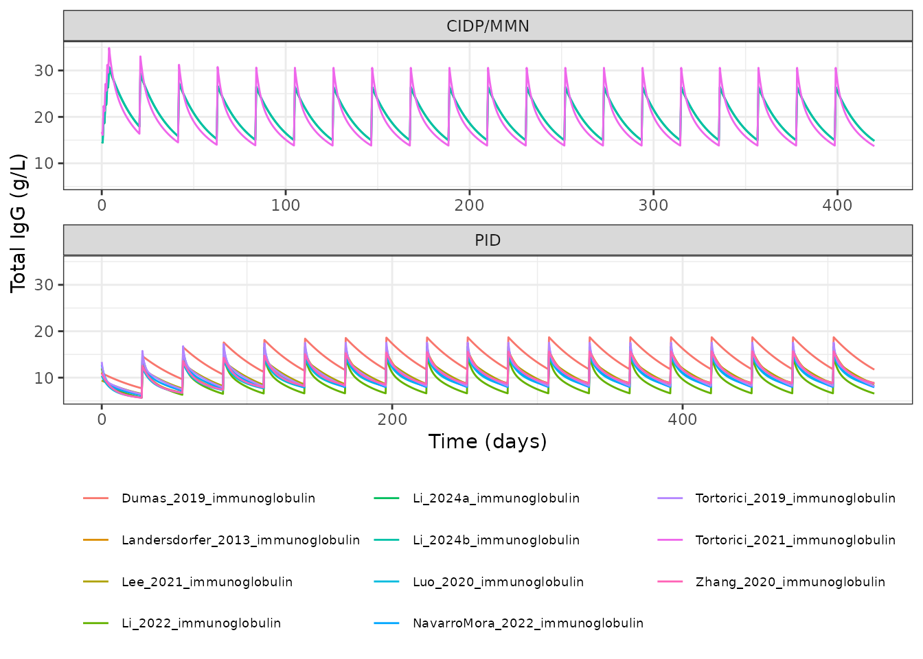
Replicates Figure 2A of van der Zeeuw 2026: population-predicted total IgG after IVIg, one curve per published model, under the review’s standardised dosing and endogenous-IgG assumptions.
Figure 2B: subcutaneous immunoglobulin
PID: 100 mg/kg weekly, loading and maintenance. CIDP and MMN: 2000 mg/kg over five days as a loading dose, then 1000 mg/kg once every three weeks.
ev_sc_pid <-
  rxode2::et(amt = 0.100 * wt_kg, cmt = "depot", ii = 7, addl = 4 * n_cycles)
t_sc_pid <- seq(0, 7 * (4 * n_cycles + 1), by = 0.5)

ev_sc_imm <-
  rxode2::et(amt = 0.400 * wt_kg, cmt = "depot", ii = 1, addl = 4) |>
  rxode2::et(amt = 1.000 * wt_kg, cmt = "depot", time = 21, ii = 21,
             addl = n_cycles)
t_sc_imm <- seq(0, 21 * (n_cycles + 2), by = 0.5)
sim_sc <- do.call(rbind, lapply(has_sc, function(m) {
  ind <- indication[[m]]
  common_cols(
    if (ind == "PID") {
      solve_typical(m, ev_sc_pid, t_sc_pid, endogenous_igg[[ind]])
    } else {
      solve_typical(m, ev_sc_imm, t_sc_imm, endogenous_igg[[ind]])
    }
  )
}))
#> ℹ change initial estimate of `bl_igg` to `4`
#> ℹ parameter labels from comments will be replaced by 'label()'
#> ℹ change initial estimate of `bl_igg` to `4`
#> ℹ omega/sigma items treated as zero: 'etalcl', 'etalvc'
#> ℹ parameter labels from comments will be replaced by 'label()'
#> ℹ change initial estimate of `bl_igg` to `4`
#> ℹ omega/sigma items treated as zero: 'etalcl', 'etalq', 'etalvc', 'etalvp', 'etalfdepot', 'etalka'
#> ℹ parameter labels from comments will be replaced by 'label()'
#> ℹ change initial estimate of `bl_igg` to `4`
#> ℹ omega/sigma items treated as zero: 'etalcl', 'etalq', 'etalvc', 'etalvp', 'etalfdepot', 'etalka'
#> ℹ parameter labels from comments will be replaced by 'label()'
#> ℹ change initial estimate of `bl_igg` to `4`
#> ℹ omega/sigma items treated as zero: 'etalcl', 'etalvc'
#> ℹ parameter labels from comments will be replaced by 'label()'
#> ℹ change initial estimate of `bl_igg` to `4`
#> ℹ omega/sigma items treated as zero: 'etalcl', 'etalvc', 'etalka'
#> ℹ parameter labels from comments will be replaced by 'label()'
#> ℹ change initial estimate of `bl_igg` to `10`
#> ℹ omega/sigma items treated as zero: 'etalcl', 'etalvc'

sim_sc$indication <- indication[sim_sc$model]
ggplot(sim_sc, aes(time, Cc, colour = model)) +
  geom_line() +
  facet_wrap(~indication, scales = "free_x", ncol = 1) +
  labs(x = "Time (days)", y = "Total IgG (g/L)", colour = NULL) +
  theme_bw() +
  theme(legend.position = "bottom", legend.text = element_text(size = 7)) +
  guides(colour = guide_legend(ncol = 3))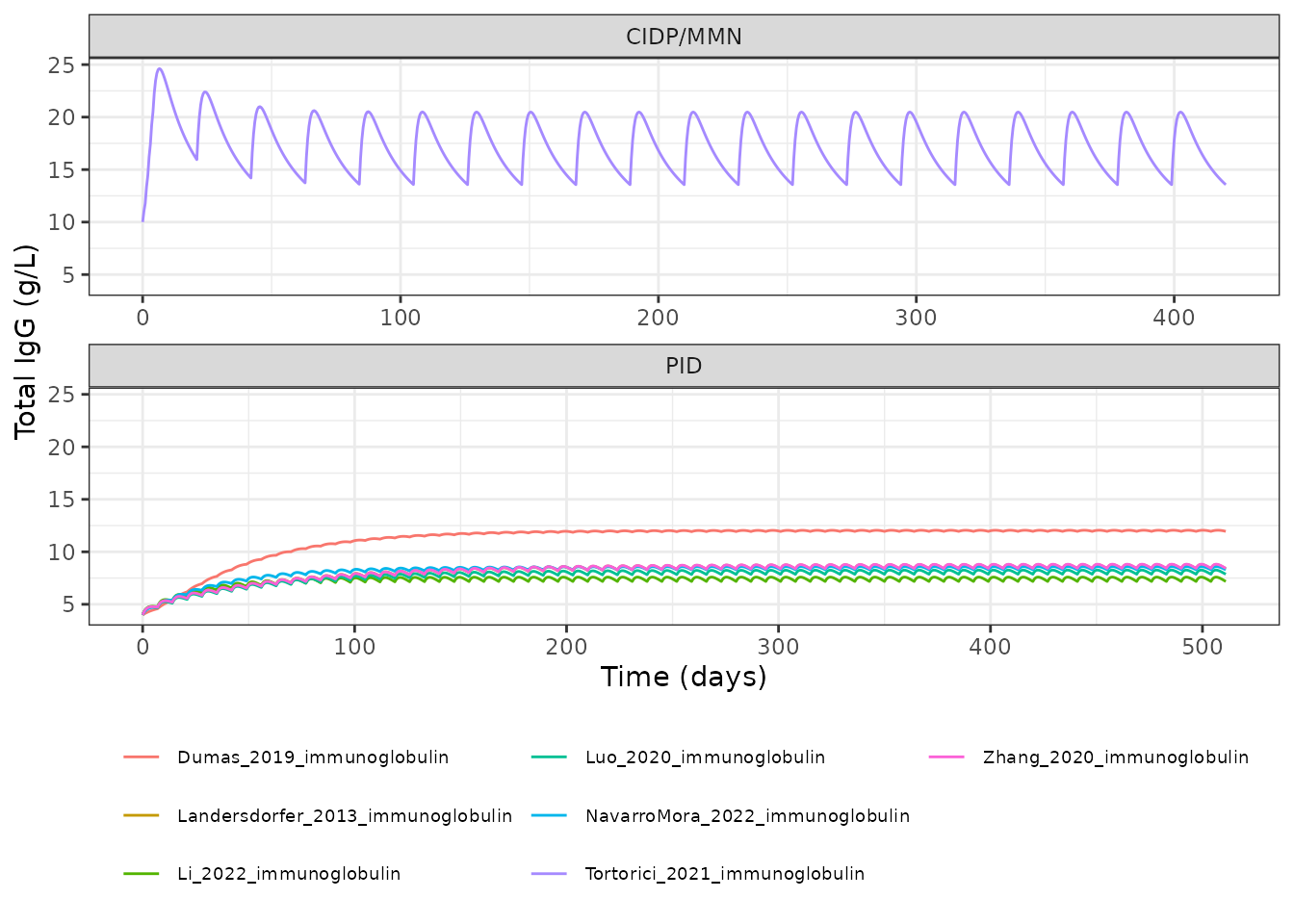
Replicates Figure 2B of van der Zeeuw 2026: population-predicted total IgG after SCIg. Only the seven models fitted to subcutaneous data are shown.
Qualitative claims from the review
The review makes three comparative claims about these panels (section 3.2.3). Each is measured against the simulation rather than taken on trust. Two reproduce; the third does not, and that discrepancy is discussed below the table.
# Steady-state window: the final maintenance interval of each profile.
ss_window <- function(d, tau) {
  tmax <- max(d$time)
  dplyr::filter(d, time >= tmax - tau, time <= tmax)
}

pid_iv_sd <- sim_iv |>
  dplyr::filter(indication == "PID") |>
  dplyr::group_by(model) |>
  dplyr::group_modify(~ ss_window(.x, 28)) |>
  dplyr::summarise(trough = min(Cc), .groups = "drop")

pid_sc_sd <- sim_sc |>
  dplyr::filter(indication == "PID") |>
  dplyr::group_by(model) |>
  dplyr::group_modify(~ ss_window(.x, 7)) |>
  dplyr::summarise(trough = min(Cc), .groups = "drop")

# Claim 1 (section 3.2.3): IVIg profiles in PID show NOTABLE between-model
# variability, whereas SCIg profiles show only MINOR differences.
cv_iv <- sd(pid_iv_sd$trough) / mean(pid_iv_sd$trough)
cv_sc <- sd(pid_sc_sd$trough) / mean(pid_sc_sd$trough)

# Claim 2 (section 3.2.3): IgG concentrations after SCIg are MORE STABLE over
# time than after IVIg. Measured as peak-to-trough swing in the last interval.
swing <- function(d, tau) {
  w <- ss_window(d, tau)
  (max(w$Cc) - min(w$Cc)) / min(w$Cc)
}
swing_iv <- sim_iv |>
  dplyr::filter(indication == "PID") |>
  dplyr::group_by(model) |>
  dplyr::summarise(s = swing(dplyr::cur_data_all(), 28), .groups = "drop")
#> Warning: There was 1 warning in `dplyr::summarise()`.
#> ℹ In argument: `s = swing(dplyr::cur_data_all(), 28)`.
#> ℹ In group 1: `model = "Dumas_2019_immunoglobulin"`.
#> Caused by warning:
#> ! `cur_data_all()` was deprecated in dplyr 1.1.0.
#> ℹ Please use `pick()` instead.
swing_sc <- sim_sc |>
  dplyr::filter(indication == "PID") |>
  dplyr::group_by(model) |>
  dplyr::summarise(s = swing(dplyr::cur_data_all(), 7), .groups = "drop")

# Claim 3 (section 3.2.3): immune-mediated-disease concentrations are HIGHER
# than PID concentrations, reflecting dose and assumed endogenous IgG.
imm_mean <- sim_iv |>
  dplyr::filter(indication == "CIDP/MMN") |>
  dplyr::group_by(model) |>
  dplyr::group_modify(~ ss_window(.x, 21)) |>
  dplyr::summarise(trough = min(Cc), .groups = "drop")

# The between-model spread is also computed on the SAME six models in both
# arms, so that "route" is not confounded with "which models happen to report
# subcutaneous data".
paired <- intersect(pid_iv_sd$model, pid_sc_sd$model)
cv_paired <- function(d) {
  x <- d$trough[d$model %in% paired]
  sd(x) / mean(x)
}

tibble::tibble(
  Claim = c(
    "SCIg profiles are flatter over time than IVIg (section 3.2.3)",
    "Immune-mediated troughs exceed PID troughs (section 3.2.3)",
    "IVIg between-model spread exceeds SCIg (section 3.2.3)"
  ),
  Measured = c(
    sprintf("median peak-to-trough swing: IVIg %.0f%% vs SCIg %.0f%%",
            100 * median(swing_iv$s), 100 * median(swing_sc$s)),
    sprintf("median trough: immune-mediated %.1f vs PID %.1f g/L",
            median(imm_mean$trough), median(pid_iv_sd$trough)),
    sprintf("CV of trough, all models: IVIg %.1f%% vs SCIg %.1f%%; paired on the same %d models: %.1f%% vs %.1f%%",
            100 * cv_iv, 100 * cv_sc, length(paired),
            100 * cv_paired(pid_iv_sd), 100 * cv_paired(pid_sc_sd))
  ),
  Reproduces = c(
    median(swing_iv$s) > median(swing_sc$s),
    median(imm_mean$trough) > median(pid_iv_sd$trough),
    cv_iv > cv_sc
  )
) |>
knitr::kable()| Claim | Measured | Reproduces |
|---|---|---|
| SCIg profiles are flatter over time than IVIg (section 3.2.3) | median peak-to-trough swing: IVIg 80% vs SCIg 5% | TRUE |
| Immune-mediated troughs exceed PID troughs (section 3.2.3) | median trough: immune-mediated 14.8 vs PID 8.4 g/L | TRUE |
| IVIg between-model spread exceeds SCIg (section 3.2.3) | CV of trough, all models: IVIg 16.9% vs SCIg 19.2%; paired on the same 6 models: 19.7% vs 19.2% | FALSE |
# Only the two claims that reproduce are asserted. These are typical-value
# (deterministic) solves, not a random cohort, so exact assertions are the
# right kind here -- there is no sampling noise for a bound to absorb.
stopifnot(
  median(swing_iv$s) > median(swing_sc$s),
  median(imm_mean$trough) > median(pid_iv_sd$trough)
)
The third claim does not reproduce, and the reason is informative. The review writes that the IVIg panel “demonstrated notable variability” while the SCIg panel showed “only minor differences”. Measured as the between-model coefficient of variation of the steady-state trough, the two routes are indistinguishable – and this holds whether all models are used or the comparison is paired on the six models that report both routes. What actually differs by an order of magnitude is the within-profile peak-to-trough swing: roughly 80% for IVIg against 5% for SCIg.
So the visual impression the review describes is real, but it is produced by each IVIg curve sweeping through a wide sawtooth rather than by the models disagreeing with one another more under IVIg. The models disagree about the trough by roughly 17-20% regardless of route. This is a claim about the review’s reading of its own figure, not a defect in any packaged model, and it does not affect any parameter value.
PKNCA validation
The review reports no non-compartmental analysis, so there is no published NCA table to compare against. Instead PKNCA is used to drive an exact structural gate.
For any linear model at steady state, the area under the exogenous concentration-time curve over one dosing interval satisfies
This identity involves no approximation, so a tight bound is
appropriate: a mis-transcribed clearance, bioavailability or reference
weight in any of the twelve files breaks it immediately, while correct
files agree to solver tolerance. Crucially, it also exercises the
derived clearance of the two models parameterised on an
elimination rate constant, where CL = Kel * Vc.
# Per-model typical clearance at the standardised patient, derived from the
# model's own parameters rather than re-entered by hand.
typical_cl <- function(model_name) {
  mod <- rxode2::rxode(readModelDb(model_name))
  if (any(!is.na(mod$iniDf$neta1))) mod <- rxode2::zeroRe(mod)
  ev <- rxode2::et(amt = 1, cmt = "central") |> rxode2::et(c(0, 1))
  s <- rxode2::rxSolve(
    mod, ev,
    params = c(WT = wt_kg, LBM = lbm_kg, DIS_SAD = 0, FORM_IG_HYALURONIDASE = 0),
    returnType = "data.frame"
  )
  # `cl` is a model variable in ten of the twelve; the two Kel-parameterised
  # models expose `kel` and `vc` instead.
  if ("cl" %in% names(s)) s$cl[1] else s$kel[1] * s$vc[1]
}

gate_one <- function(model_name, sim, tau, dose_g, fbio) {
  d <- sim[sim$model == model_name, ]
  bl <- endogenous_igg[[indication[[model_name]]]]
  tmax <- max(d$time)
  w <- d[d$time >= tmax - tau & d$time <= tmax, ]
  conc <- data.frame(
    id = 1L,
    time = w$time,
    # EXOGENOUS concentration: the identity applies to drug-derived exposure.
    conc = w$Cc - bl
  )
  conc <- conc[!is.na(conc$conc), ]
  o_conc <- PKNCA::PKNCAconc(conc, conc ~ time | id)
  o_data <- PKNCA::PKNCAdata(
    o_conc,
    intervals = data.frame(start = min(conc$time), end = max(conc$time),
                           auclast = TRUE)
  )
  res <- as.data.frame(PKNCA::pk.nca(o_data, verbose = FALSE))
  auc <- res$PPORRES[res$PPTESTCD == "auclast"]
  cl <- typical_cl(model_name)
  tibble::tibble(
    Model = model_name,
    `AUC_tau,ss (g*day/L)` = auc,
    `CL (L/day)` = cl,
    `AUC*CL (g)` = auc * cl,
    `F*Dose (g)` = fbio * dose_g,
    `Ratio` = (auc * cl) / (fbio * dose_g)
  )
}

gate_iv_pid <- do.call(rbind, lapply(
  names(indication)[indication == "PID"],
  gate_one, sim = sim_iv, tau = 28, dose_g = 0.400 * wt_kg, fbio = 1
))
#> No dose information provided, calculations requiring dose will return NA.
#> No dose information provided, calculations requiring dose will return NA.
#> ℹ parameter labels from comments will be replaced by 'label()'
#> ℹ omega/sigma items treated as zero: 'etalcl', 'etalvc'
#> No dose information provided, calculations requiring dose will return NA.
#> ℹ parameter labels from comments will be replaced by 'label()'
#> ℹ omega/sigma items treated as zero: 'etalcl', 'etalvc'
#> No dose information provided, calculations requiring dose will return NA.
#> ℹ parameter labels from comments will be replaced by 'label()'
#> ℹ omega/sigma items treated as zero: 'etalcl', 'etalq', 'etalvc', 'etalvp', 'etalfdepot', 'etalka'
#> No dose information provided, calculations requiring dose will return NA.
#> ℹ parameter labels from comments will be replaced by 'label()'
#> ℹ omega/sigma items treated as zero: 'etalcl', 'etalq', 'etalvc', 'etalvp', 'etalfdepot', 'etalka'
#> No dose information provided, calculations requiring dose will return NA.
#> ℹ parameter labels from comments will be replaced by 'label()'
#> ℹ omega/sigma items treated as zero: 'etalcl', 'etalvc'
#> No dose information provided, calculations requiring dose will return NA.
#> ℹ parameter labels from comments will be replaced by 'label()'
#> ℹ omega/sigma items treated as zero: 'etalcl', 'etalvc'
#> No dose information provided, calculations requiring dose will return NA.
#> ℹ parameter labels from comments will be replaced by 'label()'
#> ℹ omega/sigma items treated as zero: 'etalcl', 'etalvc', 'etalka'

knitr::kable(gate_iv_pid, digits = 4)| Model | AUC_tau,ss (g*day/L) | CL (L/day) | AUC*CL (g) | F*Dose (g) | Ratio |
|---|---|---|---|---|---|
| Landersdorfer_2013_immunoglobulin | 197.1336 | 0.1420 | 27.9930 | 28 | 0.9997 |
| Dumas_2019_immunoglobulin | 303.8184 | 0.0922 | 27.9999 | 28 | 1.0000 |
| Tortorici_2019_immunoglobulin | 188.4345 | 0.1486 | 28.0069 | 28 | 1.0002 |
| Luo_2020_immunoglobulin | 172.4967 | 0.1623 | 27.9999 | 28 | 1.0000 |
| Zhang_2020_immunoglobulin | 193.8697 | 0.1444 | 27.9908 | 28 | 0.9997 |
| Lee_2021_immunoglobulin | 194.0383 | 0.1443 | 28.0000 | 28 | 1.0000 |
| Li_2022_immunoglobulin | 136.6034 | 0.2050 | 28.0034 | 28 | 1.0001 |
| NavarroMora_2022_immunoglobulin | 178.0900 | 0.1572 | 28.0037 | 28 | 1.0001 |
The same identity applied to the subcutaneous arm additionally
exercises each model’s bioavailability term, since F is no
longer 1.
f_sc <- vapply(has_sc, function(m) {
  mod <- rxode2::rxode(readModelDb(m))
  if (any(!is.na(mod$iniDf$neta1))) mod <- rxode2::zeroRe(mod)
  ev <- rxode2::et(amt = 1, cmt = "depot") |> rxode2::et(c(0, 1))
  s <- rxode2::rxSolve(
    mod, ev,
    params = c(WT = wt_kg, LBM = lbm_kg, DIS_SAD = 0, FORM_IG_HYALURONIDASE = 0),
    returnType = "data.frame"
  )
  s$fdepot[1]
}, numeric(1))
#> ℹ parameter labels from comments will be replaced by 'label()'
#> ℹ omega/sigma items treated as zero: 'etalcl', 'etalvc'
#> ℹ parameter labels from comments will be replaced by 'label()'
#> ℹ omega/sigma items treated as zero: 'etalcl', 'etalq', 'etalvc', 'etalvp', 'etalfdepot', 'etalka'
#> ℹ parameter labels from comments will be replaced by 'label()'
#> ℹ omega/sigma items treated as zero: 'etalcl', 'etalq', 'etalvc', 'etalvp', 'etalfdepot', 'etalka'
#> ℹ parameter labels from comments will be replaced by 'label()'
#> ℹ omega/sigma items treated as zero: 'etalcl', 'etalvc'
#> ℹ parameter labels from comments will be replaced by 'label()'
#> ℹ omega/sigma items treated as zero: 'etalcl', 'etalvc', 'etalka'
#> ℹ parameter labels from comments will be replaced by 'label()'
#> ℹ omega/sigma items treated as zero: 'etalcl', 'etalvc'

sc_pid <- intersect(has_sc, names(indication)[indication == "PID"])

gate_sc_pid <- do.call(rbind, lapply(sc_pid, function(m) {
  gate_one(m, sim = sim_sc, tau = 7, dose_g = 0.100 * wt_kg, fbio = f_sc[[m]])
}))
#> No dose information provided, calculations requiring dose will return NA.
#> No dose information provided, calculations requiring dose will return NA.
#> ℹ parameter labels from comments will be replaced by 'label()'
#> ℹ omega/sigma items treated as zero: 'etalcl', 'etalvc'
#> No dose information provided, calculations requiring dose will return NA.
#> ℹ parameter labels from comments will be replaced by 'label()'
#> ℹ omega/sigma items treated as zero: 'etalcl', 'etalq', 'etalvc', 'etalvp', 'etalfdepot', 'etalka'
#> No dose information provided, calculations requiring dose will return NA.
#> ℹ parameter labels from comments will be replaced by 'label()'
#> ℹ omega/sigma items treated as zero: 'etalcl', 'etalq', 'etalvc', 'etalvp', 'etalfdepot', 'etalka'
#> No dose information provided, calculations requiring dose will return NA.
#> ℹ parameter labels from comments will be replaced by 'label()'
#> ℹ omega/sigma items treated as zero: 'etalcl', 'etalvc'
#> No dose information provided, calculations requiring dose will return NA.
#> ℹ parameter labels from comments will be replaced by 'label()'
#> ℹ omega/sigma items treated as zero: 'etalcl', 'etalvc', 'etalka'

knitr::kable(gate_sc_pid, digits = 4)| Model | AUC_tau,ss (g*day/L) | CL (L/day) | AUC*CL (g) | F*Dose (g) | Ratio |
|---|---|---|---|---|---|
| Landersdorfer_2013_immunoglobulin | 32.5107 | 0.1420 | 4.6165 | 4.620 | 0.9992 |
| Dumas_2019_immunoglobulin | 56.1274 | 0.0922 | 5.1727 | 5.173 | 0.9999 |
| Luo_2020_immunoglobulin | 28.7934 | 0.1623 | 4.6738 | 4.676 | 0.9995 |
| Zhang_2020_immunoglobulin | 32.7467 | 0.1444 | 4.7279 | 4.732 | 0.9991 |
| Li_2022_immunoglobulin | 24.0616 | 0.2050 | 4.9326 | 4.935 | 0.9995 |
| NavarroMora_2022_immunoglobulin | 31.3762 | 0.1572 | 4.9337 | 4.935 | 0.9997 |
Grip-strength pharmacodynamics (Li 2024b)
The only fully-parameterised PD layer in the review. IgG in excess of baseline inhibits the deterioration of grip strength, so grip strength rises from its untreated baseline of 10.6 kg toward a treated plateau.
pd <- solve_typical("Li_2024b_immunoglobulin", ev_iv_imm, t_iv_imm,
                    endogenous_igg[["CIDP/MMN"]])
#> ℹ parameter labels from comments will be replaced by 'label()'
#> ℹ change initial estimate of `bl_igg` to `10`
#> ℹ omega/sigma items treated as zero: 'etalvc', 'etalrbase'

ggplot(pd, aes(time, gs)) +
  geom_line(colour = "steelblue") +
  geom_hline(yintercept = 10.6, linetype = "dashed") +
  geom_hline(yintercept = 10.6 + 4, linetype = "dotted") +
  labs(x = "Time (days)", y = "Grip strength (kg)") +
  theme_bw()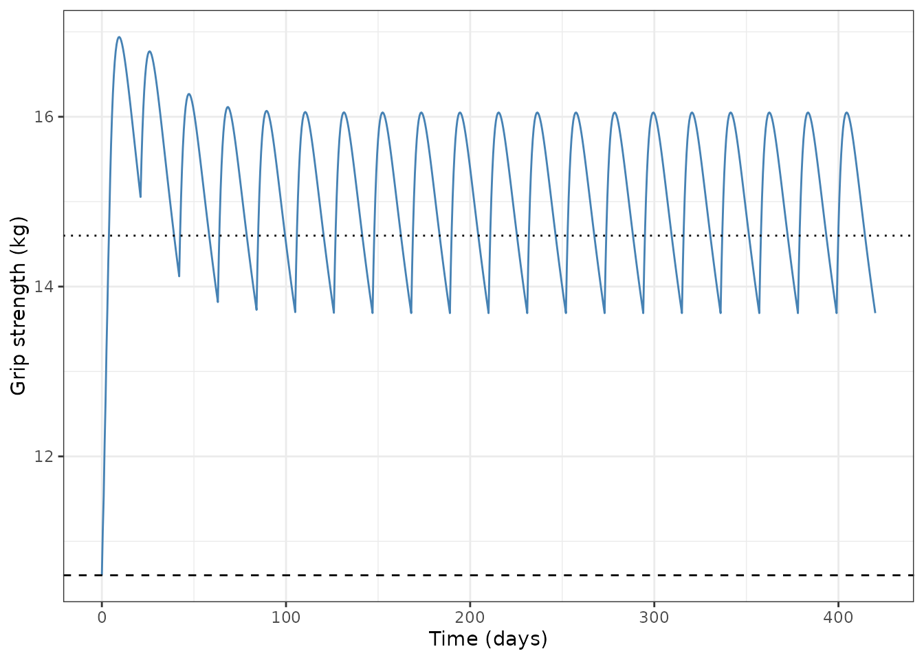
Grip strength under the MMN maintenance regimen, from the indirect-response layer of Li 2024b. The dashed line is the untreated baseline G_BASE; the dotted line is the 4 kg change the source treats as the minimal clinically meaningful improvement.
Two structural checks on the PD layer, both exact:
# 1. With no drug on board the state must hold exactly at G_BASE, since
#    kin = rbase * kout is imposed as the steady-state identity. This is the
#    check that would have caught the Supplementary Equation S1 typo
#    (Gbase = MNT/DRV rather than MNT/DTR).
# A zero-amount dose record keeps the event table well formed while delivering
# no drug, so the grip-strength state evolves with DRV identically zero.
ev_nodose <- rxode2::et(amt = 0, cmt = "central")
pd_nodose <- solve_typical("Li_2024b_immunoglobulin", ev_nodose,
                           seq(0, 200, by = 1), endogenous_igg[["CIDP/MMN"]])
#> ℹ parameter labels from comments will be replaced by 'label()'
#> ℹ change initial estimate of `bl_igg` to `10`
#> ℹ omega/sigma items treated as zero: 'etalvc', 'etalrbase'
baseline_drift <- max(abs(pd_nodose$gs - 10.6))

# 2. The treated plateau must not exceed the algebraic maximum, which is
#    G_BASE / (1 - Imax): full inhibition of the loss term.
plateau_max <- 10.6 / (1 - 0.6066)

tibble::tibble(
  Check = c("Undosed grip strength holds at G_BASE = 10.6 kg",
            "Treated grip strength stays below G_BASE/(1 - Imax)"),
  Value = c(sprintf("max drift %.3g kg", baseline_drift),
            sprintf("max %.2f kg vs bound %.2f kg", max(pd$gs), plateau_max)),
  Holds = c(baseline_drift < 1e-4, max(pd$gs) <= plateau_max)
) |>
knitr::kable()| Check | Value | Holds |
|---|---|---|
| Undosed grip strength holds at G_BASE = 10.6 kg | max drift 1.42e-14 kg | TRUE |
| Treated grip strength stays below G_BASE/(1 - Imax) | max 16.94 kg vs bound 26.94 kg | TRUE |
Assumptions and deviations
Everything below is a place where the packaged models depart from, or go beyond, what van der Zeeuw 2026 states. Because the source is a review, the list is longer than for a primary extraction, and it should be read in full before any of these twelve models is used for a decision.
Applying to all twelve
Secondary-source transcription. Every parameter comes from the review’s Table 4 or prose, not from the primary publications. Each file’s
referencefield names both. Re-verification notes per study are kept in the maintainers’ records.IIV convention. Read as apparent CV% and converted with
omega^2 = log(1 + CV^2). This follows the review’s own stated harmonisation (section 2.3) rather than being assumed.Residual-error convention.
sigma^2read as a variance, bare percentages as proportional SDs, bareAdd (g/L)values as additive SDs. See the Source trace section for the justification.-
Endogenous IgG is the weakest link. For IgG the observed concentration is endogenous plus exogenous, so the baseline is structurally load-bearing – yet Table 4 has no column for it. It is recovered from prose where possible, and the models are encoded as
Cc = central/vc + bl_igg. The provenance ofbl_iggdiffers per model and is stated in each file:Model bl_igg(g/L)Provenance Landersdorfer 2013, Luo 2020, Zhang 2020, Tortorici 2019, Navarro-Mora 2022 4 Fixed by the primary (section 3.2.1.6) Tegenge 2020 5 Fixed by the primary (section 3.2.1.6) Lee 2021 0 Endogenous IgG was subtracted from the DATA, so the DV is exogenous IgG Li 2022 6.15 Estimated by the primary; value recovered from the review’s Discussion, not Table 4 Tortorici 2021 12.5 Cohort’s observed treatment-naive median (Table 1); no parameter reported Li 2024a, Li 2024b 20.2 Cohort’s observed treatment-naive median (Table 1); CBASE was estimated but is not reported Dumas 2019 4 Not reported by the primary. The review’s own section-2.4 simulation assumption for PID The Figure 2 reproduction above overrides all of these with the review’s standardised values, which is what the review itself does.
Model-specific
-
Landersdorfer 2013 has no random effects at all.
Table 4 prints
NRin every IIV column and both residual columns, and section 3.2.1.7 confirms the error structure was not reported.propSdisfixed(0)and no etas are declared – a zero-variance eta would make OMEGA singular. The model is typical-value-only. -
Luo 2020 has no usable residual error. Table 4
footnote b: “Multiple proportional errors are reported but unclear how
they are incorporated.”
propSdisfixed(0). - Luo 2020 and Zhang 2020 share an IIV value. Both are printed with IIV on CL of exactly 36.02%. This is either coincidence or a copy error in the review; it cannot be resolved without the primaries.
- Li 2022’s residual error is flagged by the review itself. Footnote c attaches to that row alone: “Not clear whether expressed as variance or standard deviation.” The variance reading is used, for consistency with the two sibling rows in the same notation where only the variance reading gives plausible magnitudes. Under the SD reading the values would be 0.962 g/L and 10.8% instead of 0.981 g/L and 32.9%.
- Tegenge 2020’s volumes disagree between the review’s own table and prose. Table 4 gives Vc = 0.008 L and Vp = 0.055 L; the Discussion says “8.7 and 60.0 mL”. Table 4 is preferred as the parameter table. Its allometric exponent of 3.5e-07 is effectively zero, and the reference weight is not reported – 1.08 kg (the birth-weight midpoint) is used, which is numerically immaterial at that exponent.
- The Li 2024 volume exponents are not physiological. 2.23 and 2.17 on lean body mass, against a physiological expectation near 1. Transcribed as printed; these models extrapolate very badly outside the observed LBM range of roughly 40-70 kg.
- Li 2024b omits IIV on its residual error. The source estimates inter-individual variability on the PD residual term (24.5% CV). nlmixr2 has no direct encoding for IIV on sigma, so that layer is dropped.
-
Li 2024b carries an erratum. Supplementary Equation
S1 prints the steady-state identity as
Gbase = MNT/DRV.DRVthere is a typo forDTR:MNT/DRVis dimensionally inconsistent (a rate divided by a concentration is not a mass), and main-text Equation 1 evaluated atDRV = 0givesGbase = MNT/DTR. The file useskin = rbase * koutaccordingly, and the undosed-baseline check above verifies it. -
Tortorici 2019 reuses
DIS_SADfor a SID contrast. The source term is “secondary immunodeficiency”; the canonical column is “secondary antibody deficiency”, already defined with primary immunodeficiency as its reference category. The register entry was extended rather than a near-synonym minted.
Not extracted
- Tortorici 2021’s INCAT exposure-response model is not extractable. Section 3.3.2 and Supplementary Equations S3-S4 give the functional form – an Emax function of delta-IgG feeding an ordered categorical probit – but report no point estimate for Emax, EC50 or any of the probit thresholds. The only numbers given (delta-IgG of 0.8, 2.8 and 8.1 g/L at 20%, 50% and 80% of the maximum predicted probability increase) do not satisfy the Emax relation, so EC50 cannot be back-solved from them. Only the PK layer of that paper is packaged.
- Fokkink 2022 (GBS) is deliberately not extracted here. Its primary publication is to be extracted from its own open-access full text instead. The review is demonstrably unreliable for that row: it swaps the model’s volumes between Table 4 (Vc 2.87, Vp 2.65) and section 3.2.2.3 prose (Vc 2.65, Vp 2.87).
-
Lee 2024 is not yet extracted. Its six-level
disease-type covariate on Vp requires minting new
DIS_<disease>canonical columns, which is not a covariate family whose new members are accepted automatically. All of its parameters are tabulated, so it is ready to ship once those names are ratified.