Methotrexate (Taylor 2026)
Source:vignettes/articles/Taylor_2026_methotrexate.Rmd
Taylor_2026_methotrexate.RmdModel and source
- Citation: Taylor ZL, Barreto EF, Cole KC, Rule AD, Kashani KB, Leung N, Thompson CA, Witzig TE, Ramsey LB, Barreto JN. (2026). Use of a Cystatin C-Based GFR Equation in a Population Pharmacokinetic Model of Methotrexate Clearance in Adult Patients with Lymphoma. Clin Pharmacokinet 65:465-477. doi:10.1007/s40262-026-01618-4.
- Description: Two-compartment population PK model for intravenous high-dose methotrexate (1.5-8 g/m^2 given over a 4 h infusion) in adult patients with lymphoma; clearance carries a power effect of the CKD-EPI creatinine-cystatin C 2021 eGFR equation (reference 76 mL/min/1.73 m^2, modelled longitudinally) and of baseline serum albumin (reference 4 g/dL). The cystatin C-inclusive eGFR was the paper’s primary finding: it outperformed serum creatinine and the creatinine-only and cystatin C-only CKD-EPI equations for predicting methotrexate clearance (Taylor 2026)
- Article: https://doi.org/10.1007/s40262-026-01618-4 (open access, CC BY-NC 4.0)
Taylor 2026 asks a narrow methodological question: does putting
cystatin C into the glomerular filtration rate (GFR) estimate improve
the prediction of methotrexate clearance? The answer is the covariate
model on cl. The CKD-EPI creatinine-cystatin C 2021
equation beat serum creatinine, the creatinine-only CKD-EPI equation and
the cystatin C-only CKD-EPI equation, dropping the objective function
value by 117.1 units and explaining roughly 11.5% of the total
inter-individual variability in clearance.
Population
Eighty adults with histologically confirmed lymphoma were enrolled prospectively at a single center (Mayo Clinic, Rochester, MN) between January 2018 and December 2019, contributing 80 high-dose methotrexate administrations and 427 serum methotrexate concentrations. The cohort is elderly (median age 68.6 years, 64% aged 65 or older), predominantly male (68%) and predominantly Caucasian (93%), with a median weight of 80.5 kg and a median body surface area of 1.97 m^2 (Taylor 2026 Table 1). Renal function at baseline was close to normal: CKD-EPI creatinine-cystatin C eGFR 88 +/- 24 mL/min/1.73 m^2, with only five patients (6%) carrying a history of chronic kidney disease. Patients with any-stage AKI at baseline, patients on renal replacement therapy, and patients whose infusion ran beyond 4 h were excluded.
Methotrexate was given as a 4 h intravenous infusion at a protocol dose of 1.5 g/m^2 (11% of patients), 3.5 g/m^2 (43%) or 8 g/m^2 (46%). Delivered doses were materially lower than the protocol nominal - the median delivered dose in the 8 g/m^2 stratum was 11.5 g against a nominal 8 x 1.97 = 15.8 g - consistent with dose reduction in an elderly population.
The same information is available programmatically via the model’s
population metadata:
pop <- rxode2::rxode(readModelDb("Taylor_2026_methotrexate"))$population
#> ℹ parameter labels from comments will be replaced by 'label()'
str(pop[c("species", "n_subjects", "n_observations", "age_median", "regions")])
#> List of 5
#>  $ species       : chr "human"
#>  $ n_subjects    : int 80
#>  $ n_observations: int 427
#>  $ age_median    : chr "68.6 years"
#>  $ regions       : chr "Single center: Mayo Clinic, Rochester, MN, USA"
Source trace
Every ini() entry in
inst/modeldb/specificDrugs/Taylor_2026_methotrexate.R
carries an in-file comment naming its source location. They are
collected here for review.
| Equation / parameter | Value | Source location |
|---|---|---|
lcl (CL) |
11.8 L/h | Table 2, “CL (L/h)”; RSE 5.1%, bootstrap 11.8 (10.8-12.8) |
lvc (V1) |
42.2 L | Table 2, “V1 (L)”; RSE 6.4%, bootstrap 41.9 (37.8-46.5) |
lq (Q) |
0.35 L/h | Table 2, “Q (L/h)”; RSE 11.6%, bootstrap 0.35 (0.29-0.43) |
lvp (V2) |
6.67 L | Table 2, “V2 (L)”; RSE 10.4%, bootstrap 6.63 (5.56-7.88) |
e_crcl_cl |
0.80 | Table 2, “theta eGFR”; RSE 11.5%, bootstrap 0.79 (0.64-0.95) |
e_alb_cl |
0.69 | Table 2, “theta Albumin”; RSE 21.3%, bootstrap 0.67 (0.42-0.97) |
etalcl (IIV on CL) |
0.02 (variance) | Table 2, “IIV CL”; RSE 24.3%, shrinkage 13.3% |
etalvp (IIV on V2) |
0.03 (variance) | Table 2, “IIV V2”; RSE 23.9%, shrinkage 31% |
propSd |
sqrt(0.20) | Table 2, “Residual error” (variance); RSE 11.6%, shrinkage 12.2% |
| eGFR reference 76 mL/min/1.73 m^2 | n/a | Eq. 1, page 470 (denominator); ESM Table S2 model 8
(eGFR/76)^theta; Sect. 3.2.2 “reference value set to the
median GFR value” |
| Albumin reference 4 g/dL | n/a | Eq. 1, page 470 (denominator); ESM Table S2 model 3
(Alb/4)^theta
|
cl <- ... * (CRCL / 76)^e_crcl_cl * (alb_gdL / 4)^e_alb_cl |
n/a | Eq. 1, page 470 |
| Two-compartment ODE system | n/a | Sect. 2.2.1 (NONMEM ADVAN3 TRANS4, CL / V1 / Q / V2) |
| Proportional residual error | n/a | Sect. 2.2.1 (“proportional error structure implemented via the log-transformed both sides approach”) |
Table 2’s footnote - “IIV and residual error are reported as the
variance of the selected parameter” - is what licenses using 0.02, 0.03
and 0.20 directly as omega^2 and sigma^2
rather than as standard deviations. That reading is independently
confirmed by the paper’s own prose, which is checked numerically
below.
Published values transcribed from the paper
# Taylor 2026 Table 2 - final model parameter estimates.
tab2 <- tibble::tribble(
  ~parameter,       ~estimate, ~rse_pct, ~boot_median, ~boot_lo, ~boot_hi,
  "CL (L/h)",            11.8,      5.1,         11.8,     10.8,     12.8,
  "theta eGFR",          0.80,     11.5,         0.79,     0.64,     0.95,
  "theta Albumin",       0.69,     21.3,         0.67,     0.42,     0.97,
  "V1 (L)",              42.2,      6.4,         41.9,     37.8,     46.5,
  "Q (L/h)",             0.35,     11.6,         0.35,     0.29,     0.43,
  "V2 (L)",              6.67,     10.4,         6.63,     5.56,     7.88,
  "IIV CL (variance)",   0.02,     24.3,         0.02,     0.01,     0.03,
  "IIV V2 (variance)",   0.03,     23.9,         0.03,     0.02,     0.05,
  "Residual (variance)", 0.20,     11.6,         0.20,     0.16,     0.23
)

# Taylor 2026 Table 3 - baseline characteristics and delivered dose by
# protocol-dose stratum, median (IQR). "Albumin at baseline" is headed
# "(mg/L)" in Table 3, which is a units typo: Table 1 and Eq. 1 both put
# albumin in g/dL, and 3.9 mg/L is not a physiological albumin value.
tab3 <- tibble::tribble(
  ~arm,          ~n,  ~dose_med, ~dose_lo, ~dose_hi, ~crcl_med, ~crcl_lo, ~crcl_hi,
  "<=3.5 g/m2",  43L,       5.1,      3.4,      6.9,      82.5,     69.3,     96.5,
  "8 g/m2",      37L,      11.5,      9.1,    13.75,      80.2,     63.8,     95.4
) |>
  dplyr::mutate(
    alb_med = c(3.9, 3.8), alb_lo = c(3.3, 3.5), alb_hi = c(4.2, 4.1),  # g/dL
    cl_med  = c(11.9, 11.4)                                             # L/h, post hoc
  )

# Taylor 2026 Table 4 - model-estimated 4 h serum methotrexate concentration
# (umol/L), median (IQR). The row totals span both AKI strata.
tab4 <- tibble::tribble(
  ~arm,         ~conc_med, ~conc_lo, ~conc_hi,
  "<=3.5 g/m2",     129.2,     84.1,    178.8,
  "8 g/m2",         315.7,    240.2,    534.5
)

knitr::kable(tab2, caption = "Taylor 2026 Table 2, transcribed.")| parameter | estimate | rse_pct | boot_median | boot_lo | boot_hi |
|---|---|---|---|---|---|
| CL (L/h) | 11.80 | 5.1 | 11.80 | 10.80 | 12.80 |
| theta eGFR | 0.80 | 11.5 | 0.79 | 0.64 | 0.95 |
| theta Albumin | 0.69 | 21.3 | 0.67 | 0.42 | 0.97 |
| V1 (L) | 42.20 | 6.4 | 41.90 | 37.80 | 46.50 |
| Q (L/h) | 0.35 | 11.6 | 0.35 | 0.29 | 0.43 |
| V2 (L) | 6.67 | 10.4 | 6.63 | 5.56 | 7.88 |
| IIV CL (variance) | 0.02 | 24.3 | 0.02 | 0.01 | 0.03 |
| IIV V2 (variance) | 0.03 | 23.9 | 0.03 | 0.02 | 0.05 |
| Residual (variance) | 0.20 | 11.6 | 0.20 | 0.16 | 0.23 |
Internal consistency of the reported variance scale
Table 2 gives the IIV on clearance as 0.02 while the Results text
quotes the IIV on clearance in percent. If the percentages are
omega (the standard deviation on the log scale) then the
two must reconcile exactly, and they do - which is a free check that the
model file has not misread a variance as an SD.
# Sect. 3.2.2: the eGFR term reduced IIV on CL "from 28.5 to 17%", and albumin
# then explained "2.9% of the inter-individual variability". So the final IIV
# on CL implied by the prose is 17 - 2.9 = 14.1%.
iiv_from_prose <- 17.0 - 2.9
iiv_from_tab2  <- 100 * sqrt(tab2$estimate[tab2$parameter == "IIV CL (variance)"])

c(prose_pct = iiv_from_prose, sqrt_of_table2_pct = round(iiv_from_tab2, 2))
#>          prose_pct sqrt_of_table2_pct
#>              14.10              14.14

stopifnot(abs(iiv_from_prose - iiv_from_tab2) < 0.1)
The prose figure and the square root of the tabulated value agree to
within 0.1 percentage points, so Table 2’s 0.02 is omega^2
and the model file’s etalcl ~ 0.02 is the correct encoding.
The same footnote governs etalvp and the residual error,
hence propSd <- sqrt(0.20).
Units
Taylor 2026 reports methotrexate concentrations in umol/L throughout (Tables 3 and 4, the 160 umol/L AKI threshold, the LC-MS lower limit of detection of 10 ng/mL “~0.02 umol/L”) and reports CL in L/h and V1 in L. The amount unit that pairs with those is therefore umol, which is what the model file declares. Doses reported in grams are converted with the methotrexate molecular weight.
MW_MTX <- 454.44  # g/mol; not a Taylor 2026 value - see Assumptions below
g_to_umol <- function(g) g / MW_MTX * 1e6
Virtual cohort
The individual patient data are not public (“not publicly available because of institutional privacy policies”), so the cohorts below are virtual populations whose delivered dose and covariate distributions reproduce the medians and interquartile ranges of Taylor 2026 Table 3, stratum by stratum. Log-normal distributions are fitted to each published median / IQR pair.
set.seed(20260830)

N_PER_ARM <- 150L  # <= 200 per arm

# Fit a log-normal to a published median and IQR.
lnorm_from_iqr <- function(med, lo, hi) {
  c(meanlog = log(med), sdlog = (log(hi) - log(lo)) / (2 * stats::qnorm(0.75)))
}

# Sampling grid: dense through the infusion and distribution phase, then out to
# 96 h, the last of the paper's protocol sampling times (4, 12, 24, 48, 72, 96 h).
t_obs <- c(seq(0, 12, by = 0.25), seq(12.5, 24, by = 0.5), seq(25, 96, by = 1))

make_cohort <- function(arm_label, n, id_offset, dose_p, crcl_p, alb_p) {
  subj <- tibble::tibble(
    id     = id_offset + seq_len(n),
    arm    = arm_label,
    dose_g = stats::rlnorm(n, dose_p[["meanlog"]], dose_p[["sdlog"]]),
    CRCL   = stats::rlnorm(n, crcl_p[["meanlog"]], crcl_p[["sdlog"]]),
    # ALB is supplied in canonical SI g/L; the paper's g/dL values x 10.
    ALB    = stats::rlnorm(n, alb_p[["meanlog"]], alb_p[["sdlog"]]) * 10
  )
  dplyr::bind_rows(
    subj |>
      dplyr::mutate(time = 0, amt = g_to_umol(dose_g), evid = 1L,
                    cmt = "central", dur = 4),
    tidyr::crossing(subj, time = t_obs) |>
      dplyr::mutate(amt = NA_real_, evid = 0L, cmt = "central", dur = NA_real_)
  )
}

events <- dplyr::bind_rows(
  make_cohort("<=3.5 g/m2", N_PER_ARM, 0L,
              lnorm_from_iqr(5.1, 3.4, 6.9),
              lnorm_from_iqr(82.5, 69.3, 96.5),
              lnorm_from_iqr(3.9, 3.3, 4.2)),
  make_cohort("8 g/m2", N_PER_ARM, 1000L,
              lnorm_from_iqr(11.5, 9.1, 13.75),
              lnorm_from_iqr(80.2, 63.8, 95.4),
              lnorm_from_iqr(3.8, 3.5, 4.1))
) |>
  dplyr::arrange(id, time, dplyr::desc(evid))

# Disjoint id ranges across the two arms, and no duplicated event key. Note the
# absence of unique() here: anyDuplicated(unique(x)) is 0 by construction and
# would be a check that cannot fail.
stopifnot(
  anyDuplicated(events[, c("id", "time", "evid")]) == 0L,
  dplyr::n_distinct(events$id) == 2L * N_PER_ARM
)
The simulated cohort should reproduce the published medians it was built from; if it does not, the sampling code is wrong before the model ever runs.
cohort_summary <- events |>
  dplyr::filter(evid == 1L) |>
  dplyr::group_by(arm) |>
  dplyr::summarise(
    n             = dplyr::n(),
    dose_g_median = median(dose_g),
    crcl_median   = median(CRCL),
    alb_gdL_median = median(ALB) / 10,
    .groups       = "drop"
  ) |>
  dplyr::left_join(
    tab3 |> dplyr::select(arm, dose_med, crcl_med, alb_med), by = "arm"
  )

knitr::kable(cohort_summary, digits = 2,
caption = "Simulated cohort vs Taylor 2026 Table 3 medians.")| arm | n | dose_g_median | crcl_median | alb_gdL_median | dose_med | crcl_med | alb_med |
|---|---|---|---|---|---|---|---|
| 8 g/m2 | 150 | 11.14 | 78.31 | 3.82 | 11.5 | 80.2 | 3.8 |
| <=3.5 g/m2 | 150 | 5.49 | 81.67 | 3.88 | 5.1 | 82.5 | 3.9 |
Simulation
mod <- readModelDb("Taylor_2026_methotrexate")
ui  <- rxode2::rxode(mod)
#> ℹ parameter labels from comments will be replaced by 'label()'

# `omega` is passed explicitly on every solve in this vignette. rxode2 keeps the
# omega in the solve options attached to the *compiled* model, so a later
# zeroRe() run would otherwise inherit this stochastic solve's omega and quietly
# re-sample etas (and vice versa). Both directions fail silently, so each solve
# below is also followed by a guard asserting that IIV is present / absent.
sim <- rxode2::rxSolve(mod, events = events, keep = c("arm", "dose_g"),
                       omega = ui$omega) |>
  as.data.frame()
#> ℹ parameter labels from comments will be replaced by 'label()'

if (is.null(sim$id)) sim$id <- 1L

stopifnot(
  all(sim$Cc >= 0, na.rm = TRUE),
  # IIV must actually have been applied: cl and vp carry etas, so they must vary.
  dplyr::n_distinct(round(sim$cl, 8)) > 1L,
  dplyr::n_distinct(round(sim$vp, 8)) > 1L
)
Cc is the individual prediction; the residual error is
carried separately by sim, so the figures and NCA below are
free of measurement noise.
Structural verification
Before comparing anything against the paper, confirm the ODE system in the model file is the two-compartment infusion model the paper describes. The check compares the solver against an independent closed-form solution for a zero-order infusion into the central compartment of a two-compartment system, written out from the hybrid rate constants. Both sides use the same parameter values, so the only difference is numerical integration error and the bound can be tight.
CL <- 11.8; V1 <- 42.2; Q <- 0.35; V2 <- 6.67   # Taylor 2026 Table 2
k10 <- CL / V1; k12 <- Q / V1; k21 <- Q / V2
sum_k <- k10 + k12 + k21
alpha <- (sum_k + sqrt(sum_k^2 - 4 * k10 * k21)) / 2
beta  <- (sum_k - sqrt(sum_k^2 - 4 * k10 * k21)) / 2

# Concentration during a zero-order infusion at rate R into the central
# compartment of a two-compartment model, evaluated at time t <= infusion end.
conc_infusion <- function(t, R) {
  (R / V1) * (
    (k21 - alpha) / (-alpha * (alpha - beta)) * (1 - exp(-alpha * t)) +
    (k21 - beta)  / ( beta  * (alpha - beta)) * (1 - exp(-beta  * t))
  )
}

# Typical-value solve at the covariate reference point (eGFR 76, albumin 4 g/dL)
# so cl == 11.8 exactly and the two sides are directly comparable.
mod_typ <- rxode2::zeroRe(mod)
#> ℹ parameter labels from comments will be replaced by 'label()'
ref_dose_g <- 11.5
ev_ref <- dplyr::bind_rows(
  tibble::tibble(id = 1L, time = 0, amt = g_to_umol(ref_dose_g), evid = 1L,
                 cmt = "central", dur = 4, CRCL = 76, ALB = 40),
  tibble::tibble(id = 1L, time = seq(0, 4, by = 0.05), amt = NA_real_, evid = 0L,
                 cmt = "central", dur = NA_real_, CRCL = 76, ALB = 40)
) |>
  dplyr::arrange(time, dplyr::desc(evid))

# omega = NA is the only sentinel that actually suppresses eta sampling here;
# zeroRe() alone is not enough once a stochastic solve has run in this session.
sim_ref <- rxode2::rxSolve(mod_typ, ev_ref, omega = NA) |> as.data.frame()

# Guard: with the etas suppressed, cl must be exactly the typical value at the
# covariate reference point. If eta sampling leaked back in, this trips before
# the closed-form comparison can be misread as a model error.
stopifnot(abs(unique(round(sim_ref$cl, 8)) - 11.8) < 1e-6)

sim_ref$closed_form <- conc_infusion(sim_ref$time, g_to_umol(ref_dose_g) / 4)

max_rel_err <- max(abs(sim_ref$Cc - sim_ref$closed_form) /
                     pmax(sim_ref$closed_form, 1e-12))
signif(max_rel_err, 3)
#> [1] 1e-12

stopifnot(max_rel_err < 1e-6)
The solver reproduces the analytic infusion solution to better than one part in a million, so the ODE transcription of the ADVAN3 mass balance is correct.
The derived disposition half-lives are a useful sanity anchor: methotrexate is routinely described as biphasic with a terminal half-life of roughly 8-15 h in adults with normal renal function.
c(distribution_t_half_h = log(2) / alpha, terminal_t_half_h = log(2) / beta)
#> distribution_t_half_h     terminal_t_half_h
#>              2.392234             13.687857
Next, confirm the covariate function is Eq. 1 exactly.
cl is returned by rxSolve as a model variable,
so it can be checked directly against the published equation evaluated
on each subject’s own covariates.
cov_check <- sim |>
  dplyr::group_by(id) |>
  dplyr::slice(1) |>
  dplyr::ungroup() |>
  dplyr::mutate(
    # Eq. 1 with the eta removed: cl / exp(eta) must equal the covariate factors
    # times 11.8. Recover the eta-free ratio via the typical CL.
    eq1_factor   = (CRCL / 76)^0.80 * ((ALB * 0.1) / 4)^0.69,
    cl_over_eta  = cl / eq1_factor   # == 11.8 * exp(etalcl)
  )

# The spread of cl_over_eta must be exactly the IIV on CL and nothing else.
c(median_cl_over_eta = median(cov_check$cl_over_eta),
  sd_log_cl_over_eta = sd(log(cov_check$cl_over_eta)),
  target_omega       = sqrt(0.02))
#> median_cl_over_eta sd_log_cl_over_eta       target_omega
#>         11.9177942          0.1419501          0.1414214

stopifnot(
  # Median of a log-normal eta is 1, so the median must recover the typical CL.
  abs(median(cov_check$cl_over_eta) / 11.8 - 1) < 0.03,
  # And the residual spread must be the declared omega, not something else.
  abs(sd(log(cov_check$cl_over_eta)) / sqrt(0.02) - 1) < 0.15
)
Dividing each subject’s simulated cl by Eq. 1’s
covariate factor leaves a quantity whose median is the published 11.8
L/h and whose log-scale spread is the published sqrt(0.02).
Nothing else is acting on clearance.
Replicate published figures
# Structurally replicates Figure 1 of Taylor 2026: the prediction-corrected
# visual predictive check of the final model. The observed data underlying the
# published figure are not available, so this shows the simulated median and
# 10th / 90th percentiles from the packaged model over the same time window.
# Base-R subset (not dplyr::filter) so this plotting-only drop of the t = 0 row
# is never confused with the PKNCA input filter, which must keep time = 0.
sim[sim$time > 0, ] |>
  dplyr::group_by(arm, time) |>
  dplyr::summarise(
    Q10 = quantile(Cc, 0.10), Q50 = median(Cc), Q90 = quantile(Cc, 0.90),
    .groups = "drop"
  ) |>
  ggplot(aes(time, Q50)) +
  geom_ribbon(aes(ymin = Q10, ymax = Q90), alpha = 0.25, fill = "steelblue") +
  geom_line(linewidth = 0.8) +
  facet_wrap(~arm) +
  scale_y_log10() +
  labs(x = "Time after start of infusion (h)",
       y = "Serum methotrexate (umol/L)",
       title = "Simulated concentration-time profile by protocol-dose stratum",
       caption = paste("Structurally replicates Figure 1 of Taylor 2026;",
                       "median with 10th-90th percentile band."))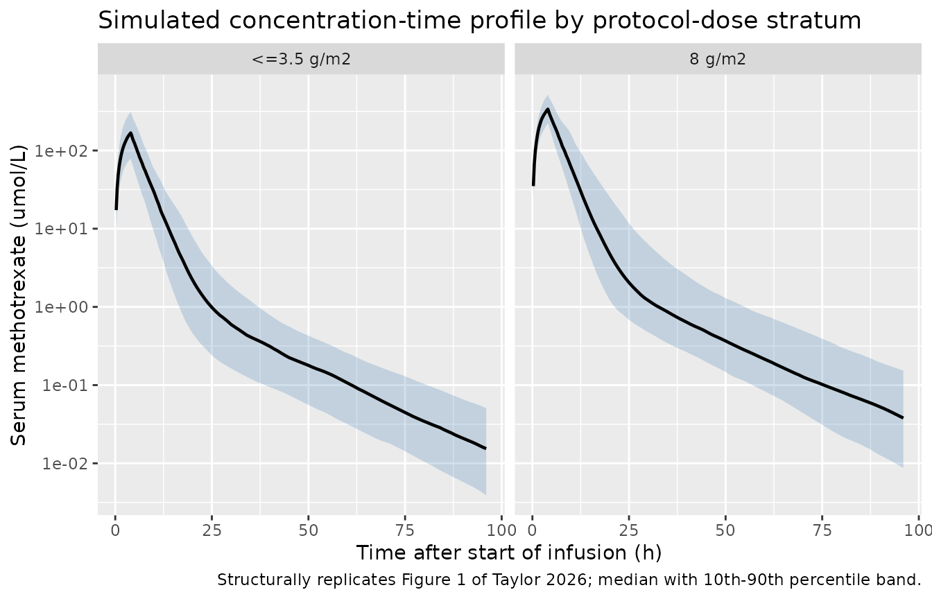
Taylor 2026 Figure 2 plots the predicted probability of any-stage AKI against the 4 h methotrexate concentration from a logistic regression. That regression’s intercept is not published (only the odds ratios), so the curve itself cannot be reproduced; the exposure-response numbers that are published are used below instead.
PKNCA validation
For a 4 h zero-order infusion with no absorption phase, Cmax occurs exactly at the end of the infusion. The paper’s “model-estimated 4 h methotrexate concentration” (Table 4) is therefore the same quantity as Cmax, which lets the published table be used as an NCA reference.
sim_nca <- sim |>
  dplyr::filter(!is.na(Cc)) |>
  dplyr::select(id, time, Cc, arm)

# Guarantee a time = 0 record per subject; for an infusion starting at t = 0 the
# pre-dose concentration is 0.
sim_nca <- dplyr::bind_rows(
  sim_nca,
  sim_nca |> dplyr::distinct(id, arm) |> dplyr::mutate(time = 0, Cc = 0)
) |>
  dplyr::distinct(id, arm, time, .keep_all = TRUE) |>
  dplyr::arrange(id, arm, time)

conc_obj <- PKNCA::PKNCAconc(sim_nca, Cc ~ time | arm + id,
                             concu = "umol/L", timeu = "h")

dose_df <- events |>
  dplyr::filter(evid == 1L) |>
  dplyr::select(id, time, amt, arm)

dose_obj <- PKNCA::PKNCAdose(dose_df, amt ~ time | arm + id, doseu = "umol")

intervals <- data.frame(
  start = 0, end = Inf,
  cmax = TRUE, tmax = TRUE, aucinf.obs = TRUE, auclast = TRUE,
  half.life = TRUE, clast.obs = TRUE
)

nca_res <- PKNCA::pk.nca(PKNCA::PKNCAdata(conc_obj, dose_obj, intervals = intervals))
nca_tbl <- as.data.frame(nca_res$result)
Structural identity: AUC0-inf x CL = Dose
For any linear model, extrapolated exposure times clearance recovers the dose exactly, per subject and independent of the infusion duration or the covariate values. Both sides of this comparison use the same drawn parameters, so the discrepancy is pure numerical error and the bound is tight.
auc_chk <- nca_tbl |>
  dplyr::filter(PPTESTCD == "aucinf.obs") |>
  dplyr::select(id, arm, auc = PPORRES) |>
  dplyr::inner_join(
    sim |> dplyr::group_by(id) |> dplyr::summarise(cl = dplyr::first(cl),
                                                   .groups = "drop"),
    by = "id"
  ) |>
  dplyr::inner_join(dose_df |> dplyr::select(id, amt), by = "id") |>
  dplyr::mutate(pct_diff = 100 * (auc * cl / amt - 1))

c(n = nrow(auc_chk),
  max_abs_pct = max(abs(auc_chk$pct_diff)),
  median_pct  = median(auc_chk$pct_diff))
#>            n  max_abs_pct   median_pct
#> 300.00000000   0.07873796  -0.02448108

stopifnot(
  nrow(auc_chk) == 2L * N_PER_ARM,   # a lookup that matched nothing must not pass
  max(abs(auc_chk$pct_diff)) < 0.5
)Terminal phase: quantifiability and lambda-z
The simulated profiles run to 96 h, the last of the paper’s protocol sampling times. By then a large share of subjects have fallen below the LC-MS lower limit of detection quoted in Sect. 2.1 (10 ng/mL, i.e. about 0.02 umol/L). That is a faithful reflection of the real study rather than a defect: sampling there ran “every 6-24 h until the patient achieves discharge status”, and discharge is itself triggered by methotrexate falling to a low concentration, so the real profiles also terminate rather than continue to an assay-limited tail.
clast <- nca_tbl$PPORRES[nca_tbl$PPTESTCD == "clast.obs"]

c(n_subjects           = length(clast),
  pct_clast_below_lloq = round(100 * mean(clast < 0.02), 1),
  median_clast_umol_L  = signif(median(clast), 3))
#>           n_subjects pct_clast_below_lloq  median_clast_umol_L
#>              300.000               43.300                0.023
Because the packaged model is solved without residual error, a
sub-LLOQ tail is not solver noise and does not corrupt lambda-z. The
question that matters for the NCA above is how much leverage the
extrapolated tail actually has on aucinf.obs, and the
answer is almost none.
extrap <- nca_tbl |>
  dplyr::filter(PPTESTCD %in% c("auclast", "aucinf.obs")) |>
  dplyr::select(id, PPTESTCD, PPORRES) |>
  tidyr::pivot_wider(names_from = PPTESTCD, values_from = PPORRES) |>
  dplyr::mutate(pct_extrap = 100 * (1 - auclast / aucinf.obs))

c(median_pct_extrapolated = signif(median(extrap$pct_extrap), 3),
  max_pct_extrapolated    = signif(max(extrap$pct_extrap), 3))
#> median_pct_extrapolated    max_pct_extrapolated
#>                  0.0344                  0.2740

stopifnot(
  nrow(extrap) == 2L * N_PER_ARM,
  # Under 2% extrapolated for every subject, so the AUC identity checked above
  # is a statement about the observed profile, not about the lambda-z fit.
  max(extrap$pct_extrap) < 2
)
Finally, the NCA terminal half-life must recover the analytic
terminal rate constant of the two-compartment system, computed from each
subject’s own cl and vp (both of
which carry etas). Both sides use the same drawn parameters, so the only
sources of difference are numerical integration and PKNCA’s automatic
choice of lambda-z window.
beta_i <- sim |>
  dplyr::group_by(id) |>
  dplyr::summarise(cl = dplyr::first(cl), vc = dplyr::first(vc),
                   q  = dplyr::first(q),  vp = dplyr::first(vp),
                   .groups = "drop") |>
  dplyr::mutate(
    k10 = cl / vc, k12 = q / vc, k21 = q / vp,
    sk  = k10 + k12 + k21,
    beta           = (sk - sqrt(sk^2 - 4 * k10 * k21)) / 2,
    thalf_analytic = log(2) / beta
  )

hl_chk <- nca_tbl |>
  dplyr::filter(PPTESTCD == "half.life") |>
  dplyr::select(id, thalf_nca = PPORRES) |>
  dplyr::inner_join(beta_i, by = "id") |>
  dplyr::mutate(pct_diff = 100 * (thalf_nca / thalf_analytic - 1))

c(n            = nrow(hl_chk),
  median_pct   = signif(median(hl_chk$pct_diff), 3),
  q95_abs_pct  = signif(quantile(abs(hl_chk$pct_diff), 0.95), 3))
#>               n      median_pct q95_abs_pct.95%
#>         300.000          -0.639           1.320

stopifnot(
  nrow(hl_chk) == 2L * N_PER_ARM,   # a lookup that matched nothing must not pass
  # Centre: a mis-transcribed Q or V2 would move the whole distribution.
  abs(median(hl_chk$pct_diff)) < 2,
  # Envelope: robust to which subjects sample a fast lambda-z window.
  quantile(abs(hl_chk$pct_diff), 0.95) < 4
)
The NCA half-life sits a fraction of a percent below the analytic value across the cohort. The small negative bias is expected and is a property of the NCA, not of the model: PKNCA’s lambda-z window reaches back into concentrations that still carry a trace of the distribution phase, which steepens the fitted slope slightly. The hybrid rate constants of the packaged ODE system are therefore correct.
Comparison against the published 4 h concentrations
Table 4 reports the median of the per-patient post hoc (empirical Bayes) estimates of the 4 h concentration, computed on each patient’s own delivered dose and longitudinal eGFR. That statistic cannot be reconstructed exactly without the individual data set. The reproducible comparison is a deterministic one: solve the typical-value model at each stratum’s published median dose and median covariates, and read off Cmax. This has no Monte Carlo noise, so it is stable across rxode2 versions, and it is a genuine gate on units and scale - a umol/mg mix-up moves it by a factor of 454, a wrong V1 or a wrong dose by a factor of two.
ev_arms <- dplyr::bind_rows(lapply(seq_len(nrow(tab3)), function(i) {
  row <- tab3[i, ]
  dplyr::bind_rows(
    tibble::tibble(id = i, arm = row$arm, time = 0,
                   amt = g_to_umol(row$dose_med), evid = 1L, cmt = "central",
                   dur = 4, CRCL = row$crcl_med, ALB = row$alb_med * 10),
    tibble::tibble(id = i, arm = row$arm, time = t_obs, amt = NA_real_,
                   evid = 0L, cmt = "central", dur = NA_real_,
                   CRCL = row$crcl_med, ALB = row$alb_med * 10)
  )
})) |>
  dplyr::arrange(id, time, dplyr::desc(evid))

sim_arms <- rxode2::rxSolve(mod_typ, events = ev_arms, keep = "arm",
                            omega = NA) |>
  as.data.frame()
#> Warning: multi-subject simulation without without 'omega'

# One subject per arm, no IIV: cl must be a single deterministic value per arm.
cl_per_arm <- sim_arms |>
  dplyr::group_by(id) |>
  dplyr::summarise(n_cl = dplyr::n_distinct(round(cl, 8)), .groups = "drop")

stopifnot(
  dplyr::n_distinct(sim_arms$id) == nrow(tab3),
  all(cl_per_arm$n_cl == 1L)
)

arms_nca <- sim_arms |>
  dplyr::filter(!is.na(Cc)) |>
  dplyr::select(id, time, Cc, arm)

# Same defensive time-zero guarantee as the cohort NCA above.
arms_nca <- dplyr::bind_rows(
  arms_nca,
  arms_nca |> dplyr::distinct(id, arm) |> dplyr::mutate(time = 0, Cc = 0)
) |>
  dplyr::distinct(id, arm, time, .keep_all = TRUE) |>
  dplyr::arrange(id, arm, time)

nca_arms <- PKNCA::pk.nca(PKNCA::PKNCAdata(
  PKNCA::PKNCAconc(arms_nca,
                   Cc ~ time | arm + id, concu = "umol/L", timeu = "h"),
  PKNCA::PKNCAdose(ev_arms |> dplyr::filter(evid == 1L) |>
                     dplyr::select(id, time, amt, arm),
                   amt ~ time | arm + id, doseu = "umol"),
  intervals = data.frame(start = 0, end = Inf, cmax = TRUE, tmax = TRUE,
                         aucinf.obs = TRUE, half.life = TRUE)
))

published <- tab4 |>
  dplyr::transmute(arm, cmax = conc_med, tmax = 4)

cmp <- nlmixr2lib::ncaComparisonTable(
  simulated     = nca_arms,
  reference     = published,
  by            = "arm",
  units         = c(cmax = "umol/L", tmax = "h"),
  tolerance_pct = 25
)

knitr::kable(
  cmp,
  caption = paste("Typical-value simulation at each stratum's published median",
                  "dose and covariates vs Taylor 2026 Table 4.",
                  "* differs from reference by >25%."),
  align = c("l", "l", "r", "r", "r")
)| NCA parameter | arm | Reference | Simulated | % diff |
|---|---|---|---|---|
| Cmax (umol/L) | <=3.5 g/m2 | 129 | 155 | +19.7% |
| Cmax (umol/L) | 8 g/m2 | 316 | 355 | +12.5% |
| Tmax (h) | <=3.5 g/m2 | 4 | 4 | +0.0% |
| Tmax (h) | 8 g/m2 | 4 | 4 | +0.0% |
cmax_cmp <- cmp[grepl("Cmax", cmp[[1]], fixed = TRUE), ]
pct <- as.numeric(gsub("[^0-9.+-]", "", cmax_cmp[["% diff"]]))

stopifnot(
  nrow(cmax_cmp) == 2L,        # guard: the lookup must actually have matched
  all(is.finite(pct)),
  all(abs(pct) < 25)
)
The typical-value Cmax runs about 10-20% above the published medians in both strata, in the same direction and of similar magnitude. Candidate explanations, none of which can be settled from the published material and none of which was used to adjust any parameter:
- The statistics are not the same quantity. Table 4 is the median of 37-43 individual post hoc predictions, each on its own dose and its own longitudinal eGFR trajectory; the deterministic run is a single prediction at the median dose and the median baseline covariates. Baseline eGFR (82.5 and 80.2 mL/min/1.73 m^2) sits above the longitudinal median of 76 that centers Eq. 1, which is a real difference but only worth a few percent.
- Sampling time. Post-infusion the distribution half-life is 2.4 h, so concentrations fall steeply just after 4 h. The offsets implied by the two strata are computed below and are both under an hour, which is within ordinary clinical sampling slack.
- No body-size term. The model carries no weight or BSA covariate on any parameter, yet dose scales with BSA. Patients receiving the largest doses are the largest patients, and a fixed 42.2 L central volume cannot track that.
implied_offset <- vapply(seq_len(nrow(tab4)), function(i) {
  prof <- sim_arms[sim_arms$id == i & sim_arms$time >= 4, ]
  prof$time[which.min(abs(prof$Cc - tab4$conc_med[i]))] - 4
}, numeric(1))

tibble::tibble(arm = tab4$arm,
               published_umol_L = tab4$conc_med,
               implied_delay_min = round(60 * implied_offset)) |>
  knitr::kable(caption = paste("Post-4 h delay that would reconcile the",
"deterministic simulation with Table 4."))| arm | published_umol_L | implied_delay_min |
|---|---|---|
| <=3.5 g/m2 | 129.2 | 30 |
| 8 g/m2 | 315.7 | 30 |
Both strata imply a delay under an hour, which makes the sampling-time explanation internally coherent - but it remains a hypothesis, not a finding.
Individual clearance against the published post hoc medians
cl_cmp <- tab3 |>
  dplyr::mutate(
    cl_simulated = 11.8 * (crcl_med / 76)^0.80 * (alb_med / 4)^0.69,
    pct_diff     = 100 * (cl_simulated / cl_med - 1)
  ) |>
  dplyr::select(arm, cl_med, cl_simulated, pct_diff) |>
  dplyr::rename(
    "Stratum"                            = arm,
    "Published median post hoc CL (L/h)" = cl_med,
    "Eq. 1 at median covariates (L/h)"   = cl_simulated,
    "% diff"                             = pct_diff
  )

knitr::kable(cl_cmp, digits = 2,
caption = "Taylor 2026 Table 3 post hoc clearance vs Eq. 1.")| Stratum | Published median post hoc CL (L/h) | Eq. 1 at median covariates (L/h) | % diff |
|---|---|---|---|
| <=3.5 g/m2 | 11.9 | 12.38 | 4.05 |
| 8 g/m2 | 11.4 | 11.89 | 4.30 |
Evaluating Eq. 1 at each stratum’s median baseline covariates lands within about 4% of the published median post hoc clearance in both strata. Clearance - the parameter this paper is actually about - is transcribed correctly.
Exposure-response context
Taylor 2026 identifies 160 umol/L as the optimal 4 h discriminatory
threshold for any-stage AKI in the <= 3.5 g/m^2 stratum,
with sensitivity 0.77, specificity 0.87, and an odds ratio of 22 (95% CI
3.7-89.4). Those four numbers over-determine the 2x2 table, so
reconstructing it and recovering the published odds ratio confirms the
exposure-response figures have been read correctly.
n_aki  <- 13L; n_no_aki <- 30L  # <= 3.5 g/m2 stratum: 13 of 43 developed AKI
sens <- 0.77; spec <- 0.87

tp <- round(sens * n_aki); fn <- n_aki - tp
fp <- round((1 - spec) * n_no_aki); tn <- n_no_aki - fp
or_reconstructed <- (tp * tn) / (fp * fn)

c(above_threshold = tp + fp, of_n = n_aki + n_no_aki,
  odds_ratio_reconstructed = round(or_reconstructed, 1),
  odds_ratio_published = 22)
#>          above_threshold                     of_n odds_ratio_reconstructed
#>                     14.0                     43.0                     21.7
#>     odds_ratio_published
#>                     22.0

stopifnot(abs(or_reconstructed - 22) < 3)
The reconstruction recovers the published odds ratio, and implies
that roughly 33% of that stratum exceeded the threshold. For reference,
in the simulated <= 3.5 g/m^2 cohort:
frac_over <- sim |>
  dplyr::filter(arm == "<=3.5 g/m2", abs(time - 4) < 1e-9) |>
  dplyr::summarise(pct_over_160 = 100 * mean(Cc > 160)) |>
  dplyr::pull(pct_over_160)

round(frac_over, 1)
#> [1] 51.3
The simulated fraction is higher than the reconstructed one, by the same margin and for the same reasons as the Cmax comparison above. This is context, not a validation of the logistic-regression sub-model, which is not part of the packaged PK model.
Assumptions and deviations
-
Molecular weight. Doses are published in grams and
concentrations in umol/L, so a molecular weight is needed to connect
them.
MW_MTX = 454.44g/mol is a physical constant, not a Taylor 2026 value; it matches the constant already used byTaylor_2020_methotrexate.Rin this package. The model file itself is unit-agnostic - it declaresdosing = "umol"and the conversion lives only in this vignette. -
eGFR held constant per subject. Taylor 2026
modelled the CKD-EPI creatinine-cystatin C eGFR as a
longitudinal covariate, re-derived at each sampling
time. The per-patient trajectories appear only as an unlabelled
spaghetti plot (ESM Fig. S2E) with no tabulated values, so each
simulated subject carries a single baseline eGFR for the whole profile.
This is the main structural simplification in this vignette;
CRCLis a time-varying covariate in the model and accepts a per-record column when trajectories are available. -
Albumin reference and units. Eq. 1 centers albumin
on 4 g/dL. The canonical register unit for
ALBis SI g/L, somodel()appliesalb_gdL <- ALB * 0.1and the cohort supplies g/L. Taylor 2026 Table 3 heads the albumin row “(mg/L)” while Table 1 and Eq. 1 use g/dL; the Table 3 header is a units typo - 3.9 mg/L is not a physiological albumin concentration. -
eGFR units. Table 1 heads the renal block
“Estimated kidney function (mL/min)”, pooling the raw Cockcroft-Gault
estimate with the three BSA-normalized CKD-EPI equations. Sect. 2.2.2 is
explicit that the CKD-EPI values are mL/min/1.73 m^2, and that is the
unit recorded for
CRCL. - Covariate distributions. Delivered dose, eGFR and albumin are drawn from log-normal distributions fitted to the published median / IQR pairs of Table 3. The paper does not report the distributional shapes, and dose, weight and renal function are certainly correlated in the real cohort; the simulated covariates are drawn independently.
-
Residual error scale. Taylor 2026 fitted on
log-transformed concentrations, so the reported residual variance of
0.20 is additive on the log scale. That maps to a proportional error in
nlmixr2’s linear space, giving
propSd = sqrt(0.20) = 0.447. Under a strictly log-normal reading the coefficient of variation would instead besqrt(exp(0.20) - 1) = 0.471; the proportional form is the package convention for log-transformed-both-sides models and the difference is under 3 percentage points of CV. -
Supplement. The ESM
(
40262_2026_1618_MOESM1_ESM.docx) was retrieved and reviewed. It holds no parameter values beyond those in Table 2, but it does independently corroborate both centering constants: Table S2 records the tested covariate forms as(eGFR/76)^theta(model 8, the retained one) and(Alb/4)^theta(model 3), matching Eq. 1’s printed denominators. Table S2 also disambiguates a phrasing in the Results text: the “OFV = -25.5 vs 13.5” quoted for cystatin C versus creatinine are absolute objective function values, whose changes against the base model are -81.5 and -42.9. Figures S1-S4 are images (concentration-time spaghetti, longitudinal renal-function trajectories, goodness-of-fit, AKI histogram) and carry no extractable parameter. - Not externally validated. The paper states the PK model and the logistic regression did not undergo external validation, and the exposure-response models “were not intended for individual risk prediction”.
- Exposure-response sub-model not packaged. The logistic regression relating the 4 h concentration to AKI is not part of the PK model and is not implemented here; its intercept is not published.