Budesonide Entocort EC dissolution (Han 2023)
Source:vignettes/articles/Han_2023_budesonide_dissolution.Rmd
Han_2023_budesonide_dissolution.RmdModel and source
Han 2023 built a Simcyp whole-body PBPK model of the budesonide controlled-release capsule Entocort EC in healthy volunteers and Crohn’s disease patients, and used it for virtual bioequivalence trials comparing local gut and systemic exposure across eight virtual test formulations. The formulation enters that PBPK model as a Weibull dissolution function fitted to the in vitro dissolution profile of the Entocort EC pellets (Equation 4, Table 2, Supplementary Table S1). That dissolution function is packaged here.
- Model: In vitro (biorelevant FaSSIF dissolution of Entocort EC pellets). Weibull dissolution (release) function for the budesonide controlled-release capsule Entocort EC, fitted by the authors to the in vitro dissolution profile of the pellets and used as the formulation input of their Simcyp whole-body PBPK model. Release-only: there is no budesonide disposition. The undissolved drug in the pellets (depot) dissolves with the Weibull hazard; the outputs are the cumulative amount dissolved (released) and the instantaneous dissolution rate. The Simcyp PBPK model the function fed (multilayer gut wall ADAM absorption, Rodgers and Rowland tissue distribution, CYP3A4 clearance) is not part of this model. The paper’s six virtual test formulations (Table 2) are reproduced by overriding lra and lgam1.
- Citation: Han C, Sun T, Chirumamilla SK, Bois FY, Xu M, Rostami-Hodjegan A. Understanding Discordance between In Vitro Dissolution, Local Gut and Systemic Bioequivalence of Budesonide in Healthy and Crohn’s Disease Patients through PBPK Modeling. Pharmaceutics. 2023;15(9):2237. doi:10.3390/pharmaceutics15092237. Weibull form from Equation (4); Entocort EC parameter values from Supplementary Table S1 (to five significant figures; Table 2 prints the same fit rounded to 3.12 and 0.94).
- Article: https://doi.org/10.3390/pharmaceutics15092237
- Supplement (Table S1): https://www.mdpi.com/article/10.3390/pharmaceutics15092237/s1
The PBPK model itself is not part of the package. Its tissue distribution uses Simcyp’s Rodgers and Rowland method with only a global Kp scalar (0.8) reported, its hepatic and gut clearance is a CYP3A4 intrinsic clearance per pmol of enzyme that needs Simcyp’s enzyme abundances and organ scalars, and its absorption runs through Simcyp’s eight-segment multilayer gut wall (M-ADAM) model with regional absorption scalars applied to internal permeabilities. None of the organ volumes, blood flows, tissue partition coefficients or enzyme abundances behind those inputs are printed, so the PBPK model cannot be reproduced from the publication.
Population
The dissolution function is an in vitro curve fit, not a population
model. The source profile is the Entocort EC pellet dissolution in
fasted-state simulated intestinal fluid (FaSSIF) reported by Effinger et
al. (Eur J Pharm Sci 2021;157:105617; Han 2023 reference 22), sampled
every 0.5 h up to 6 h. Because the measured profile had not reached 100%
at its last sampling time, the authors added a 100% point at the end of
the profile (Section 2.4.4). There is no inter-individual variability
and no residual error. The same information is available
programmatically via
readModelDb("Han_2023_budesonide_dissolution")()$population.
The eight virtual test formulations of the paper were built by hand from that reference profile. Six shift the percent dissolved by a fixed number of percentage points at every sampling time (+20%, +10%, +5%, +3%, -5%, -10%, capped at 100%) and were refitted to the same Weibull function (Table 2). The other two keep the Entocort EC profile and change only the enteric-coating trigger pH (5 or 6 instead of 5.5), which affects release in vivo but not the in vitro dissolution curve.
Source trace
| Equation / parameter | Value | Source location |
|---|---|---|
Weibull dissolution,
F = Fmax * (1 - exp(-(t - Tlag)^beta / alpha))
|
n/a | Equation (4) |
lra (ra = alpha^(-1/beta)) |
log(3.1196^(-1/0.93998)) = log(0.298) 1/h | Table S1 (Alpha = 3.1196, Beta = 0.93998); Table 2 (alpha = 3.12) |
lgam1 (beta) |
log(0.93998) | Table S1 (Beta = 0.93998); Table 2 (beta = 0.94) |
lfdepot (Fmax / 100) |
log(1), fixed | Table S1 and Table 2 (Fmax = 100) |
Tlag |
0 | not reported; see Assumptions |
| Virtual formulations (alpha, beta) | +20% (1.53, 0.87); +10% (2.14, 0.89); +5% (2.56, 0.91); +3% (2.77, 0.92); -5% (3.90, 1.01); -10% (5.01, 1.09) | Table 2 |
Similarity factor f2
|
Equation (3) | Section 2.4.4 |
| Residual error, inter-individual variability | none | deterministic curve fit |
The canonical Weibull release input in nlmixr2lib leaves the fraction
still undissolved as S(t) = exp(-(ra * t)^gam1). Matching
it to Equation (4) gives gam1 = beta and
ra = alpha^(-1/beta), so the lra value is
computed from the published alpha and beta,
not printed directly.
Simulation
One 3 mg Entocort EC capsule is dosed into depot at the
start of dissolution, and the dissolved amount is read from the
released sink. The virtual formulations reuse the same
model with lra and lgam1 overridden by the
Table 2 values.
mod <- rxode2::rxode2(readModelDb("Han_2023_budesonide_dissolution"))

dose_mg <- 3
# Rounded so the 0.5 h sampling times below match exactly.
obs_h <- sort(unique(round(c(seq(0, 12, by = 0.05), 11, 12), 4)))
ev <- dplyr::bind_rows(
  data.frame(id = 1L, time = 0, amt = dose_mg, cmt = "depot", evid = 1L),
  data.frame(id = 1L, time = obs_h, amt = 0, cmt = "released", evid = 0L)
)

# Table 2 Weibull parameters, in the alpha / beta form of Equation (4).
# Entocort EC uses the full-precision Table S1 values carried by the model.
formulations <- tibble::tribble(
  ~formulation,   ~shift, ~alpha,  ~beta,   ~f2_published,
  "Entocort EC",  0,      3.1196,  0.93998, NA,
  "+20%",         20,     1.53,    0.87,    36.1,
  "+10%",         10,     2.14,    0.89,    50.8,
  "+5%",          5,      2.56,    0.91,    65.5,
  "+3%",          3,      2.77,    0.92,    75.8,
  "-5%",          -5,     3.90,    1.01,    65.5,
  "-10%",         -10,    5.01,    1.09,    50.8
) |>
  dplyr::mutate(formulation = factor(formulation, levels = formulation))

solve_formulation <- function(alpha, beta) {
  sim <- rxode2::rxSolve(
    mod,
    events = ev,
    params = c(lra = log(alpha^(-1 / beta)), lgam1 = log(beta)),
    rtol = 1e-10, atol = 1e-12
  )
  as.data.frame(sim) |>
    dplyr::transmute(time, released, releaseRate, pct = 100 * released / dose_mg)
}

sim <- formulations |>
  dplyr::rowwise() |>
  dplyr::reframe(formulation, shift, alpha, beta, solve_formulation(alpha, beta))
Check against the published closed form
The ODE solution must reproduce Equation (4) evaluated at the published parameters. Both sides use the same values, so the only difference is integration error and a tight bound is appropriate.
weibull_pct <- function(t, alpha, beta) 100 * (1 - exp(-t^beta / alpha))

cf <- sim |>
  dplyr::mutate(pct_closed = weibull_pct(time, alpha, beta), diff = pct - pct_closed)

cf |>
  dplyr::group_by(formulation) |>
  dplyr::summarise(max_abs_diff = max(abs(diff))) |>
  dplyr::rename("Formulation" = formulation, "Max |ODE - Equation (4)| (points)" = max_abs_diff) |>
knitr::kable(digits = 6)| Formulation | Max |ODE - Equation (4)| (points) |
|---|---|
| Entocort EC | 4.0e-06 |
| +20% | 4.9e-05 |
| +10% | 2.3e-05 |
| +5% | 1.2e-05 |
| +3% | 9.0e-06 |
| -5% | 0.0e+00 |
| -10% | 1.0e-06 |
The model dissolves the whole capsule: at 24 h the undissolved
fraction of the Entocort EC profile is 0.0017, so tad()
restarting at a second daily capsule does not lose drug from the
first.
Replicate Figure 2
The points below were digitised by the maintainers from the thick blue reference profile of Figure 2 (sampling times 0.5 to 6 h, with the 100% end point). The lines are the packaged Weibull model at the Table 2 parameters.
# Entocort EC reference profile, digitised from Han 2023 Figure 2 (percent
# dissolved). The final point is the 100% assumed by the authors; the figure
# draws it at 11 h while Section 2.4.4 says 12 h.
ref_digitised <- data.frame(
  time = c(seq(0.5, 6, by = 0.5), 12),
  pct = c(14.8, 28.6, 38.8, 47.0, 53.3, 59.1, 64.3, 68.8, 72.4, 76.4, 79.5, 84.4, 100)
)
ggplot(sim, aes(time, pct, colour = formulation, linetype = shift < 0)) +
  geom_line(linewidth = 0.8) +
  geom_point(
    data = ref_digitised, aes(time, pct), inherit.aes = FALSE,
    colour = "black", size = 1.8
  ) +
  scale_linetype_manual(values = c(`FALSE` = "solid", `TRUE` = "dashed"), guide = "none") +
  coord_cartesian(xlim = c(0, 12), ylim = c(0, 100)) +
  labs(
    x = "Time (h)", y = "Dissolved (%)", colour = NULL,
    title = "Weibull dissolution of Entocort EC and virtual formulations",
    caption = "Replicates Figure 2 of Han 2023. Points: Entocort EC profile digitised from Figure 2."
  ) +
  theme_bw()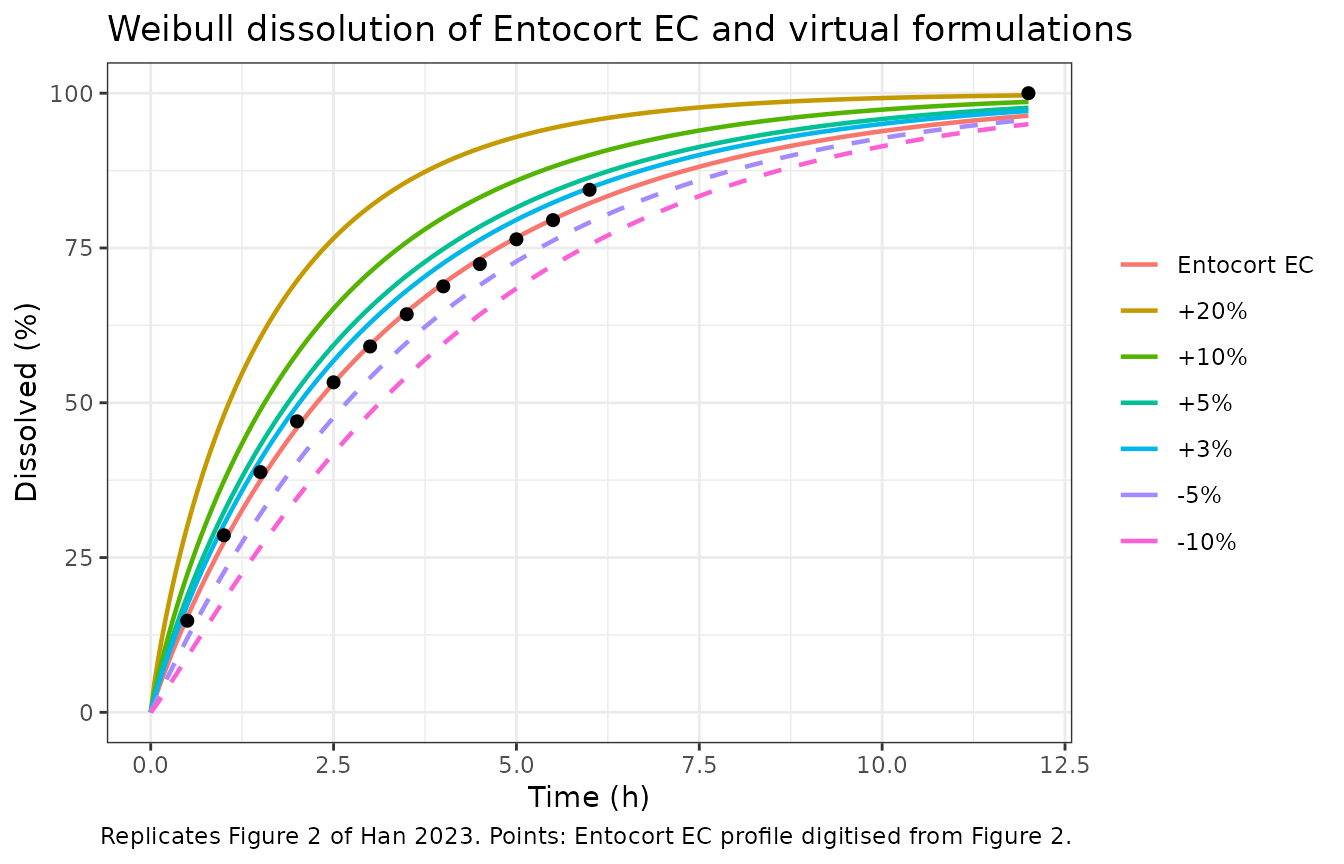
Known-answer checks
The packaged curve, the digitised data and the published table are tied together in three ways. All three are deterministic.
- The packaged Entocort EC curve passes through the digitised reference profile. Digitising error is about one percentage point. The bound applies to the twelve measured points (0.5 to 6 h). The 100% end point was added by the authors rather than measured, and the fitted Weibull reaches only about 96% at 12 h, so it is shown in the table but not bounded.
sampling_h <- c(seq(0.5, 6, by = 0.5), 12)
ref_model <- sim |>
  dplyr::filter(formulation == "Entocort EC", round(time, 4) %in% sampling_h) |>
  dplyr::transmute(time = round(time, 4), pct_model = pct)
chk_ref <- dplyr::inner_join(ref_digitised, ref_model, by = "time") |>
  dplyr::mutate(diff = pct_model - pct)

chk_ref |>
  dplyr::rename(
    "Time (h)" = time, "Digitised (%)" = pct,
    "Model (%)" = pct_model, "Model - digitised (points)" = diff
  ) |>
knitr::kable(digits = 1)| Time (h) | Digitised (%) | Model (%) | Model - digitised (points) |
|---|---|---|---|
| 0.5 | 14.8 | 15.4 | 0.6 |
| 1.0 | 28.6 | 27.4 | -1.2 |
| 1.5 | 38.8 | 37.5 | -1.3 |
| 2.0 | 47.0 | 45.9 | -1.1 |
| 2.5 | 53.3 | 53.2 | -0.1 |
| 3.0 | 59.1 | 59.4 | 0.3 |
| 3.5 | 64.3 | 64.7 | 0.4 |
| 4.0 | 68.8 | 69.3 | 0.5 |
| 4.5 | 72.4 | 73.2 | 0.8 |
| 5.0 | 76.4 | 76.7 | 0.3 |
| 5.5 | 79.5 | 79.6 | 0.1 |
| 6.0 | 84.4 | 82.2 | -2.2 |
| 12.0 | 100.0 | 96.4 | -3.6 |
measured <- chk_ref$time <= 6
stopifnot(
  nrow(chk_ref) == length(sampling_h),
  median(abs(chk_ref$diff[measured])) < 1.5,
  max(abs(chk_ref$diff[measured])) < 3,
  abs(chk_ref$diff[!measured] + 3.6) < 0.5
)-
Refitting Equation (4) to the digitised profile recovers the
published alpha and beta. This also settles the form of the
Weibull: with
alphadividingt^beta, as printed, the refit lands on the Table S1 values; readingalphaas a time scale inside the power,(t / alpha)^beta, would needalphanear 3.3 instead.
refit <- stats::nls(
  pct ~ 100 * (1 - exp(-time^beta / alpha)),
  data = ref_digitised,
  start = list(alpha = 3, beta = 1)
)
refit_coef <- stats::coef(refit)
data.frame(
  parameter = c("alpha", "beta"),
  published = c(3.1196, 0.93998),
  refit_to_digitised = unname(refit_coef[c("alpha", "beta")])
) |>
  dplyr::mutate(ratio = refit_to_digitised / published) |>
  dplyr::rename(
    "Parameter" = parameter, "Table S1" = published,
    "Refit to digitised Figure 2" = refit_to_digitised, "Ratio" = ratio
  ) |>
knitr::kable(digits = 3)| Parameter | Table S1 | Refit to digitised Figure 2 | Ratio |
|---|---|---|---|
| alpha | 3.12 | 3.100 | 0.994 |
| beta | 0.94 | 0.943 | 1.003 |
stopifnot(abs(refit_coef[["alpha"]] / 3.1196 - 1) < 0.03, abs(refit_coef[["beta"]] / 0.93998 - 1) < 0.03)-
The similarity factors of Table 2 follow from the virtual
profiles. Equation (3) applied to the digitised reference and
the shifted profiles (reference plus the shift at each of the twelve
measured sampling times, capped at 100%, and the same 100% end point as
the reference) must reproduce the published f2 values; applied to the
packaged Weibull curves of each virtual formulation it must land close
to them, which tests the Table 2
alpha/betapairs. The mean shift of each Weibull curve over 0.5 to 6 h must also match the formulation’s nominal shift.
f2 <- function(r, t) 50 * log10(100 / sqrt(1 + mean((r - t)^2)))

model_at <- function(form) {
  sim |>
    dplyr::filter(formulation == form, round(time, 4) %in% sampling_h) |>
    dplyr::arrange(time) |>
    dplyr::pull(pct)
}
ref_curve <- model_at("Entocort EC")

chk_f2 <- formulations |>
  dplyr::filter(formulation != "Entocort EC") |>
  dplyr::rowwise() |>
  dplyr::mutate(
    f2_digitised = f2(ref_digitised$pct, pmin(c(ref_digitised$pct[1:12] + shift, 100), 100)),
    f2_weibull = f2(ref_curve, model_at(as.character(formulation))),
    mean_shift_weibull = mean(model_at(as.character(formulation))[1:12] - ref_curve[1:12])
  ) |>
  dplyr::ungroup()

chk_f2 |>
  dplyr::select(formulation, shift, f2_published, f2_digitised, f2_weibull, mean_shift_weibull) |>
  dplyr::rename(
    "Formulation" = formulation, "Nominal shift (points)" = shift,
    "f2, Table 2" = f2_published, "f2, digitised profiles" = f2_digitised,
    "f2, packaged Weibull curves" = f2_weibull,
    "Mean Weibull shift, 0.5-6 h (points)" = mean_shift_weibull
  ) |>
knitr::kable(digits = 1)| Formulation | Nominal shift (points) | f2, Table 2 | f2, digitised profiles | f2, packaged Weibull curves | Mean Weibull shift, 0.5-6 h (points) |
|---|---|---|---|---|---|
| +20% | 20 | 36.1 | 36.1 | 36.3 | 19.2 |
| +10% | 10 | 50.8 | 50.8 | 50.2 | 10.1 |
| +5% | 5 | 65.5 | 65.5 | 64.3 | 5.2 |
| +3% | 3 | 75.8 | 75.8 | 75.1 | 3.1 |
| -5% | -5 | 65.5 | 65.5 | 67.1 | -4.5 |
| -10% | -10 | 50.8 | 50.8 | 51.9 | -9.3 |
stopifnot(
  all(abs(chk_f2$f2_digitised - chk_f2$f2_published) < 0.3),
  all(abs(chk_f2$f2_weibull - chk_f2$f2_published) < 2.5),
  all(abs(chk_f2$mean_shift_weibull - chk_f2$shift) < 1.5)
)
The f2 values computed from the Weibull curves sit within about 1.6 units of Table 2, as expected for a three-parameter fit to a hand-shifted profile; the digitised profiles reproduce Table 2 to the printed precision.
Dissolution milestones
The paper does not tabulate dissolution times, so these are reported
for reference only, from the closed-form inverse of Equation (4):
t_p = (-alpha * log(1 - p))^(1/beta).
milestones <- formulations |>
  dplyr::mutate(
    t50 = (-alpha * log(1 - 0.5))^(1 / beta),
    t632 = alpha^(1 / beta),
    t80 = (-alpha * log(1 - 0.8))^(1 / beta),
    t90 = (-alpha * log(1 - 0.9))^(1 / beta)
  )
milestones |>
  dplyr::select(formulation, alpha, beta, t50, t632, t80, t90) |>
  dplyr::rename(
    "Formulation" = formulation, "alpha" = alpha, "beta" = beta,
    "t50% (h)" = t50, "t63.2% (h)" = t632, "t80% (h)" = t80, "t90% (h)" = t90
  ) |>
knitr::kable(digits = 2)| Formulation | alpha | beta | t50% (h) | t63.2% (h) | t80% (h) | t90% (h) |
|---|---|---|---|---|---|---|
| Entocort EC | 3.12 | 0.94 | 2.27 | 3.35 | 5.57 | 8.15 |
| +20% | 1.53 | 0.87 | 1.07 | 1.63 | 2.82 | 4.25 |
| +10% | 2.14 | 0.89 | 1.56 | 2.35 | 4.01 | 6.00 |
| +5% | 2.56 | 0.91 | 1.88 | 2.81 | 4.74 | 7.03 |
| +3% | 2.77 | 0.92 | 2.03 | 3.03 | 5.08 | 7.49 |
| -5% | 3.90 | 1.01 | 2.68 | 3.85 | 6.16 | 8.79 |
| -10% | 5.01 | 1.09 | 3.13 | 4.39 | 6.79 | 9.43 |
Noncompartmental analysis
Not applicable. The model has no disposition, so there is no concentration profile to analyse with PKNCA; the paper’s plasma and gut-segment Cmax and AUC values (Tables 6 and 7) are outputs of the Simcyp PBPK model, which is not packaged. The validation above uses the dissolution profile the function was fitted to and the similarity factors derived from it.
Assumptions and deviations
- PBPK model not packaged. Only the formulation input (the Weibull dissolution function) is extracted. The whole-body PBPK model, the Crohn’s disease population changes (Table 4), the within-subject variability of the virtual bioequivalence trials (Table 5) and the bioequivalence heatmaps are Simcyp platform constructs whose organ-level parameters the paper does not print.
-
Weibull form. Equation (4) divides
(t - Tlag)^betabyalpha, which is Simcyp’s Weibull dissolution form. The refit of the digitised Figure 2 profile above confirms that reading. -
Lag time. Equation (4) includes
Tlag, but no value is reported for any formulation. It is taken as zero, which the publishedalphaandbetarequire to reproduce Figure 2. In vivo, the Entocort EC coating starts to dissolve only above pH 5.5 (Table 2, trigger pH), after a 0.8 h mean pellet residence time in the stomach (Table S1); both belong to the PBPK model and are not represented here, so time zero of this model is the start of dissolution, not the time of capsule ingestion. - End of the profile. Section 2.4.4 says 100% dissolution was assumed at 12 h; Figure 2 draws the 100% point at about 11 h. The f2 values do not depend on that time, and the checks above use 12 h.
-
Precision. The model uses the five-figure Table S1
values for Entocort EC; Table 2 prints the same fit rounded to
alpha = 3.12,beta = 0.94. The virtual formulations are available only at the Table 2 precision. - Figure 2 legend. The legend prints f2 = 65.6 for the +5% formulation (Table 2: 65.5) and “f2+50.8” for -10%; the Table 2 values are used.
- Trigger-pH formulations. The “pH threshold = 5” and “pH threshold = 6” formulations have the Entocort EC Weibull parameters and differ only in the in vivo trigger pH, so their in vitro dissolution curve is the reference curve.