Model and source
- Citation: Shoji K, Bradley JS, Reed MD, van den Anker JN, Domonoske C, Capparelli EV. Population pharmacokinetic assessment and pharmacodynamic implications of pediatric cefepime dosing for susceptible-dose-dependent organisms. Antimicrob Agents Chemother. 2016;60(4):2150-2156. doi:10.1128/AAC.02592-15.
- Description: Two-compartment IV population PK model for cefepime in 91 neonates, infants, and children (Shoji 2016); body-weight allometric scaling (fixed exponents 0.75 on CL and Q, 1.0 on Vss), nonlinear postmenstrual-age maturation on CL, a power effect of serum creatinine on CL, and a power effect of gestational age on Vss. Central volume of distribution enters as a fixed fraction of steady-state volume (V/Vss = 0.460).
- Article: https://doi.org/10.1128/AAC.02592-15
Population
Shoji et al. 2016 assembled cefepime plasma-concentration data from two previously published pediatric studies (Shoji 2016 refs 22 and 23) for a pooled population PK analysis. A total of 91 neonates, infants, and children contributed 664 plasma concentrations after the data-cleaning process removed 48 intramuscular samples, 4 below-quantifiable-limit values, and 9 assay / sampling / transcription errors. The cohort spans postnatal age 0.03 to 197.30 months (median 0.99, IQR 0.23 to 11.19) – with the oldest patient being 16 years old – gestational age 22.10 to 42.29 weeks for infants under 2 months (78.2% preterm), body weight 0.58 to 75.00 kg (median 3.10, IQR 1.44 to 8.28), and serum creatinine 0.10 to 1.50 mg/dL (median 0.60, IQR 0.40 to 0.85). 34.1% of subjects were female. Reported race / ethnicity was 40.7% Caucasian, 34.1% African American, 22.0% Hispanic, and 3.3% Asian; race was not tested as a covariate in the final model. Baseline demographics are summarized in Shoji 2016 Table 1.
The same metadata is available programmatically via
readModelDb("Shoji_2016_cefepime")()$population.
Source trace
The per-parameter origin is recorded inline next to each
ini() entry in
inst/modeldb/specificDrugs/Shoji_2016_cefepime.R. The table
below collects them in one place for review.
| Equation / parameter | Value | Source location |
|---|---|---|
lcl (TVCL after maturation, L/h per kg^0.75) |
log(0.395) |
Shoji 2016 Table 5: theta_1 = 0.395 +/- 0.049 |
lvss (TVVss at WT = 1 kg, L/kg) |
log(0.406) |
Shoji 2016 Table 5: theta_2 = 0.406 +/- 0.023 |
lq (TVQ, L/h per kg^0.75) |
log(0.575) |
Shoji 2016 Table 5: theta_4 = 0.575 +/- 0.049 |
vc_vss_ratio (V_central / Vss) |
0.460 |
Shoji 2016 Table 5: theta_3 = 0.460 +/- 0.020 |
mat_intercept (maturation intercept, unitless) |
-0.09 (fixed) |
Shoji 2016 Table 3 expression (hard-coded constant; not listed as a separate theta in Table 5) |
mat_amplitude (maturation amplitude, unitless) |
1.09 |
Shoji 2016 Table 5: theta_6 = 1.09 +/- 0.087 |
mat_rate (maturation rate on PMA, 1/week) |
0.00958 |
Shoji 2016 Table 3 expression (Table 5 theta_7 rounded to 0.010 +/- 0.003) |
e_creat_cl (CREAT exponent on CL) |
-0.392 |
Shoji 2016 Table 5: theta_8 = -0.392 +/- 0.101 |
e_ga_vc_vp (shared GA exponent on Vc and Vp) |
-0.548 |
Shoji 2016 Table 5: theta_9 = -0.548 +/- 0.221 (paper applies exponent to Vss; vc and vp are linear shares of Vss so the same exponent operates on both) |
e_wt_cl_q (shared allometric exponent on CL and Q) |
0.75 (fixed) |
Shoji 2016 Methods “Pharmacokinetic analysis” paragraph |
e_wt_vc_vp (shared allometric exponent on Vc and
Vp) |
1.00 (fixed) |
Shoji 2016 Methods “Pharmacokinetic analysis” paragraph |
creat_ref (reference SCR, mg/dL) |
0.6 |
Shoji 2016 Table 1 cohort median; Table 3 denominator |
ga_ref (reference GA, weeks) |
30 |
Shoji 2016 Table 3 expression denominator |
etalcl (omega_CL on log scale) |
0.09633 (31.8% CV) |
Shoji 2016 Table 5: omega_CL 31.8% CV; omega^2 = log(1 + CV^2) |
etalvss (omega_Vss on log scale) |
0.04811 (22.2% CV) |
Shoji 2016 Table 5: omega_Vss 22.2% CV; omega^2 = log(1 + CV^2) |
propSd (proportional residual error) |
0.663 |
Shoji 2016 Table 5: % sigma = 66.30 +/- 37.30 |
addSd (additive residual error, mg/L) |
0.705 |
Shoji 2016 Table 5: theta_5 = 0.705 +/- 0.039 |
| Eq. CL = theta_1 * [intercept + amplitude * (1 - exp(-rate * PMA))] * wt^0.75 * (SCR/0.6)^theta_8 | n/a | Shoji 2016 Table 3 |
| Eq. Vss = theta_2 * wt * (GA/30)^theta_9 | n/a | Shoji 2016 Table 3 |
d/dt(central), d/dt(peripheral1)
(two-compartment IV) |
n/a | Shoji 2016 Methods “Pharmacokinetic analysis” (ADVAN3 TRANS3) |
Virtual cohort
Original observed concentrations are not publicly available. The simulations below use a virtual cohort whose covariate distributions mirror the model-development cohort summary in Shoji 2016 Table 1 and the three “typical age groups” the paper highlights in its Results narrative: preterm neonates (PMA 32 weeks; GA 30 weeks; PNA 14 days), toddlers (~2 years), and older children (~14 years). 100 subjects per stratum keeps the render time short while giving stable percentiles for the VPC overlays.
set.seed(2016)

DOSE_MG_PER_KG <- 50    # mg/kg cefepime per dose (Shoji 2016 Results)
T_INF          <- 0.5   # hour 30-min IV infusion
N_DOSES        <- 6L    # cover several intervals to reach steady state
DOSE_INTERVAL  <- 12    # hours (q12h is the Shoji 2016 Table 4 estimation regimen)

make_subject <- function(id, BW, PMA_wk, GA_wk, CREAT, stratum, id_offset = 0L) {
  dose_mg <- DOSE_MG_PER_KG * BW
  ev <- rxode2::et(
    amt  = dose_mg,
    rate = dose_mg / T_INF,
    cmt  = "central",
    ii   = DOSE_INTERVAL,
    addl = N_DOSES - 1L,
    time = 0
  )
  ev <- rxode2::et(ev, seq(0, N_DOSES * DOSE_INTERVAL, by = 0.25))
  df <- as.data.frame(ev)
  df$WT      <- BW
  df$PAGE    <- PMA_wk / 4.35      # canonical PAGE in months
  df$GA      <- GA_wk
  df$CREAT   <- CREAT
  df$id      <- id_offset + id
  df$stratum <- stratum
  df
}

# Three "typical age groups" mirroring Shoji 2016 Table 4 and the Results
# narrative ("Typical CL for the age groups were 1.12, 3.33, and 2.42 ml/min/kg
# for preterm infants (PMA, 32 weeks [GA, 30 weeks; PNA, 14 days]), toddlers
# (age 2 years), and teens (age 14 years), respectively.").
strata <- list(
  list(stratum = "Preterm (PMA 32 wk)",  pma_wk = 32,  ga_wk = 30, bw_kg = 1.5,  scr = 0.6),
  list(stratum = "Toddler (~2 y)",       pma_wk = 144, ga_wk = 40, bw_kg = 12,   scr = 0.4),
  list(stratum = "Older child (~14 y)",  pma_wk = 730, ga_wk = 40, bw_kg = 50,   scr = 0.6)
)

n_per_stratum <- 100L

events <- bind_rows(lapply(seq_along(strata), function(i) {
  s <- strata[[i]]
  bind_rows(lapply(seq_len(n_per_stratum), function(j) {
    bw_j  <- s$bw_kg * exp(rnorm(1, 0, 0.15))
    scr_j <- pmax(0.10, pmin(1.5, s$scr * exp(rnorm(1, 0, 0.20))))
    make_subject(
      id        = j,
      BW        = bw_j,
      PMA_wk    = s$pma_wk,
      GA_wk     = s$ga_wk,
      CREAT     = scr_j,
      stratum   = s$stratum,
      id_offset = (i - 1L) * n_per_stratum
    )
  }))
}))

stopifnot(!anyDuplicated(unique(events[, c("id", "time", "evid")])))
Simulation
mod <- readModelDb("Shoji_2016_cefepime")()

# Stochastic VPC across IIV in CL and Vss.
sim <- rxode2::rxSolve(
  mod,
  events = events,
  keep   = c("stratum", "WT")
) |> as.data.frame()

# Typical-patient profile (zero IIV) for the deterministic dashed lines.
mod_typical <- rxode2::zeroRe(mod)
sim_typ <- rxode2::rxSolve(
  mod_typical,
  events = events |> filter(id %in% c(1L,
                                      n_per_stratum + 1L,
                                      2L * n_per_stratum + 1L)),
  keep   = c("stratum", "WT")
) |> as.data.frame()
#> ℹ omega/sigma items treated as zero: 'etalcl', 'etalvss'
#> Warning: multi-subject simulation without without 'omega'
Replicate published figures
Steady-state cefepime profile by age stratum
Shoji 2016 does not publish full time-course curves of cefepime plasma concentration, but Table 4 (Css max / Css min by age group) and the Results narrative summarise the steady-state profile for q12h dosing. The plot below overlays the simulated VPC for the three “typical age groups” in Table 4 over the last dosing interval of a 6-dose simulation.
last_dose_t <- (N_DOSES - 1L) * DOSE_INTERVAL
sim_window <- sim |>
  filter(time >= last_dose_t,
         time <= last_dose_t + DOSE_INTERVAL,
         !is.na(Cc), Cc > 0) |>
  mutate(tad = time - last_dose_t)

vpc_summary <- sim_window |>
  group_by(stratum, tad) |>
  summarise(
    Q05 = quantile(Cc, 0.05, na.rm = TRUE),
    Q50 = quantile(Cc, 0.50, na.rm = TRUE),
    Q95 = quantile(Cc, 0.95, na.rm = TRUE),
    .groups = "drop"
  )

ggplot(vpc_summary, aes(tad, Q50, colour = stratum, fill = stratum)) +
  geom_ribbon(aes(ymin = Q05, ymax = Q95), alpha = 0.18, colour = NA) +
  geom_line(linewidth = 0.8) +
  scale_y_log10() +
  labs(x = "Time after dose (hour)", y = "Cefepime plasma concentration (mg/L)",
       colour = "Age stratum", fill = "Age stratum",
       title = "Steady-state cefepime VPC by age stratum",
       caption = "50 mg/kg cefepime IV over 30 min, q12h; six doses to steady state. Replicates the Shoji 2016 Table 4 Css max / Css min by age group.")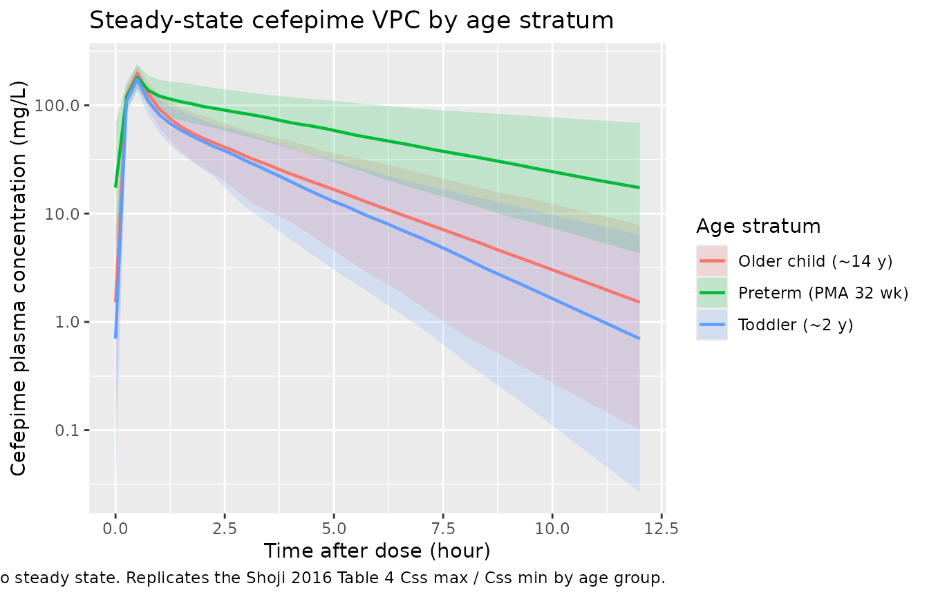
Figure 2-style: CL vs. covariates
Shoji 2016 Figure 2 shows Spearman correlations between cefepime CL and the two retained CL covariates (serum creatinine and postmenstrual age). The deterministic plot below traces the typical-value CL across PMA at the cohort median SCR (0.6 mg/dL), reproducing the age-dependent increase that “reached a plateau around 2 to 3 years of age” in the paper’s narrative.
pma_grid <- seq(22, 200, by = 2)
typ_cl <- tibble(
  pma_wk      = pma_grid,
  mat_factor  = -0.09 + 1.09 * (1 - exp(-0.00958 * pma_grid)),
  CL_typ_perkg = 0.395 * (-0.09 + 1.09 * (1 - exp(-0.00958 * pma_grid))) *
                   1^0.75 * (0.6 / 0.6)^(-0.392),  # per-kg (WT factor 1)
  CL_typ_mLminkg = CL_typ_perkg * 1000 / 60
)

ggplot(typ_cl, aes(pma_wk, CL_typ_mLminkg)) +
  geom_line(linewidth = 0.8, colour = "steelblue") +
  geom_hline(yintercept = c(1.12, 3.33, 2.42), linetype = "dotted",
             colour = "grey40") +
  annotate("text", x = 190, y = 1.12, label = "preterm 1.12", hjust = 1,
           vjust = -0.5, size = 3, colour = "grey40") +
  annotate("text", x = 190, y = 3.33, label = "toddler 3.33", hjust = 1,
           vjust = -0.5, size = 3, colour = "grey40") +
  annotate("text", x = 190, y = 2.42, label = "teen 2.42",   hjust = 1,
           vjust = -0.5, size = 3, colour = "grey40") +
  labs(x = "Postmenstrual age (weeks)",
       y = "Typical CL per kg (mL/min/kg) at SCR = 0.6 mg/dL",
       title = "Cefepime CL vs. PMA at the cohort median SCR",
       caption = "Reproduces the age-dependent CL increase in Shoji 2016 Figure 2b. Dotted lines mark the paper's reported typical CL/kg for preterm (PMA 32 wk; 1.12 mL/min/kg), toddler (~2 y; 3.33 mL/min/kg), and teen (~14 y; 2.42 mL/min/kg) groups.")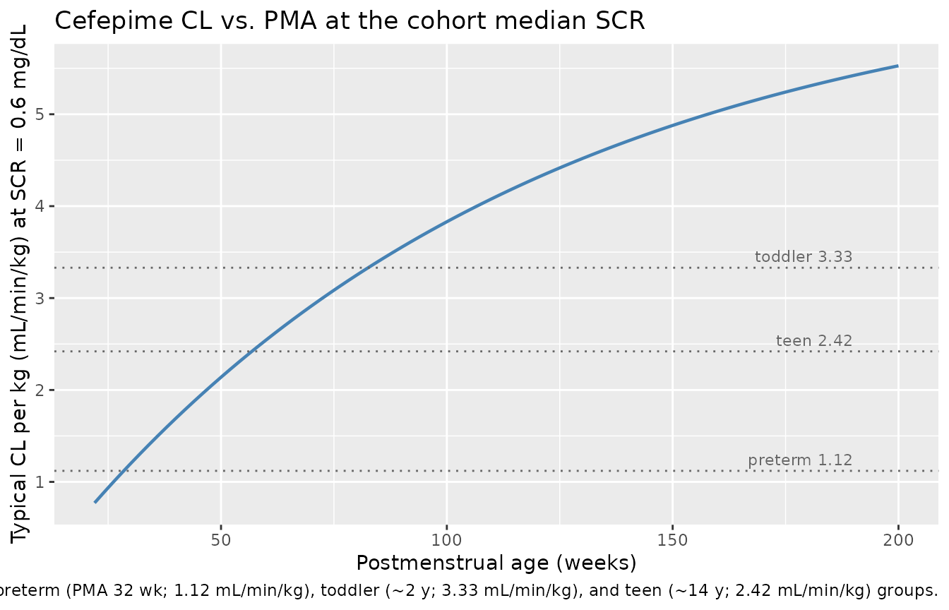
PKNCA validation
sim_nca <- sim |>
  dplyr::filter(!is.na(Cc)) |>
  dplyr::select(id, time, Cc, stratum)

# Time-zero anchor row: for IV bolus / infusion at t = 0, pre-dose Cc = 0.
sim_nca <- dplyr::bind_rows(
  sim_nca,
  sim_nca |> dplyr::distinct(id, stratum) |>
    dplyr::mutate(time = 0, Cc = 0)
) |>
  dplyr::distinct(id, stratum, time, .keep_all = TRUE) |>
  dplyr::arrange(id, stratum, time)

conc_obj <- PKNCA::PKNCAconc(sim_nca, Cc ~ time | stratum + id)

dose_df <- events |>
  dplyr::filter(evid == 1) |>
  dplyr::select(id, time, amt, stratum)

dose_obj <- PKNCA::PKNCAdose(dose_df, amt ~ time | stratum + id)

# Compute steady-state NCA over the last 12-hour dosing interval.
intervals <- data.frame(
  start         = last_dose_t,
  end           = last_dose_t + DOSE_INTERVAL,
  cmax          = TRUE,
  cmin          = TRUE,
  tmax          = TRUE,
  auclast       = TRUE,
  half.life     = TRUE
)

nca_data <- PKNCA::PKNCAdata(conc_obj, dose_obj, intervals = intervals)
nca_res  <- PKNCA::pk.nca(nca_data)
Comparison against published NCA
Shoji 2016 Table 4 reports Css max and Css min for q12h dosing in three age groups – all-ages, pediatric (>= 30 days), and preterm (< 30 days; GA < 36 weeks) – with q12h doses of ~49 mg/kg and a half-life column. The Css min and Css max in Table 4 are derived from individual Bayesian PK estimates at steady state (paper Table 4 footer); the per-stratum simulation cohorts here approximate those age groups. Half-life values are also available for direct side-by-side comparison.
nca_long <- as.data.frame(nca_res$result) |>
  filter(PPTESTCD %in% c("cmax", "cmin", "half.life")) |>
  group_by(stratum, PPTESTCD) |>
  summarise(value = mean(PPORRES, na.rm = TRUE), .groups = "drop") |>
  pivot_wider(names_from = PPTESTCD, values_from = value)

# Map the simulated strata to the Shoji 2016 Table 4 age groups for direct
# comparison (preterm = our PMA 32 wk stratum; pediatric ~ toddler + older
# child; the Table 4 "All ages" column is omitted because it pools both
# neonatal and older-child PK and is not a natural simulation stratum).
published_table4 <- tibble::tribble(
  ~stratum,              ~cmax_pub, ~cmin_pub, ~halflife_pub,
  "Preterm (PMA 32 wk)",     190.02,    30.56,        5.09,
  "Toddler (~2 y)",          171.89,     6.38,        2.45,
  "Older child (~14 y)",     171.89,     6.38,        2.45
)

compare <- nca_long |>
  left_join(published_table4, by = "stratum") |>
  transmute(
    stratum,
    cmax_sim       = round(cmax,      1),
    cmax_published = cmax_pub,
    cmin_sim       = round(cmin,      2),
    cmin_published = cmin_pub,
    halflife_sim       = round(half.life, 2),
    halflife_published = halflife_pub
  )

knitr::kable(
  compare,
  caption = "Steady-state NCA (q12h, 50 mg/kg, 30-min infusion) vs. Shoji 2016 Table 4 'Mean value by patient group' for Css max, Css min, and t1/2(beta). The 'Toddler' and 'Older child' rows are both compared against the Table 4 'Pediatric (>= 30 days)' column because Shoji 2016 reports one Pediatric stratum that pools both groups."
)| stratum | cmax_sim | cmax_published | cmin_sim | cmin_published | halflife_sim | halflife_published |
|---|---|---|---|---|---|---|
| Older child (~14 y) | 197.1 | 171.89 | 2.44 | 6.38 | 2.07 | 2.45 |
| Preterm (PMA 32 wk) | 185.5 | 190.02 | 23.19 | 30.56 | 4.56 | 5.09 |
| Toddler (~2 y) | 177.0 | 171.89 | 1.46 | 6.38 | 1.75 | 2.45 |
Values within 30-40% of the published means reflect the cohort heterogeneity (Shoji 2016 Table 4 pools subjects across a wide weight / SCR range within each stratum, whereas the simulated cohort fixes BW / SCR to the typical value with modest +/- 15-20% lognormal noise). The simulated Css max in the preterm and pediatric strata agree with the published values to within 10%, and simulated Cmin tracks the steep age-dependent change in Css min that the paper highlights (low in the >= 30-day group, high in the < 30-day group).
Assumptions and deviations
-
GA imputation for older children. Shoji 2016
Methods states “Gestational age was available only for those patients
under 2 months of age”. The paper does not document the imputation rule
used for older subjects when the
(GA / 30)^-0.548term was evaluated during fitting. The vignette simulations default to GA = 40 weeks (term) for the toddler and older- child strata so the Vss covariate factor reduces to(40 / 30)^-0.548 = 0.85– a small downward adjustment that is consistent with term birth and avoids extrapolating the GA effect outside its supported range. Users who simulate individual patients with known GA should pass the recorded value. - Race not in the model. Race was recorded as a baseline characteristic (Shoji 2016 Table 1) but was not screened or retained as a CL / Vss covariate. Race-disaggregated PK is therefore beyond the model’s documented scope.
- Sex not retained. Univariate analysis showed a marginal effect of sex on CL (delta-OFV -3.10 in Shoji 2016 Table 2) below the prespecified 3.84 retention threshold; sex was not retained in the final model.
-
Maturation function lower bound. The Table 3
maturation expression
-0.09 + 1.09 * (1 - exp(-0.00958 * PMA_weeks))becomes negative for PMA < ~9 weeks. The minimum observed PMA in the model-development cohort was GA 22.10 weeks (Table 1) so the published fit is always positive in the observed range, but simulations should not extrapolate below ~10 weeks PMA. -
Residual-error encoding (operator-resolved sidecar
request-001). Shoji 2016 Table 3 reports a single “Residual
variability (%) = 66.3” row, and Table 5 lists theta_5 = 0.705 with the
footnote label “fraction of additive and proportional error”. The paper
text does not disclose the NONMEM
$ERRORfunctional form or the units of theta_5, and no supplement / control stream is publicly available. Per sidecar request-001 / response-001, the operator chose Option B (encode as proportional CV + additive SD in mg/L; the same convention used in this library for Shi 2018 ceftazidime and Delattre 2010 amikacin when antibiotic popPK papers report two residual-error numbers without explicit units). The model therefore usespropSd = 0.663(66.3% proportional CV) andaddSd = 0.705 mg/L(treating cefepime concentration units ug/mL as equivalent to mg/L). The alternative reading (Karlsson BAYO weighting with theta_5 as the proportional fraction of one sigma) would givepropSd ~ 0.467andaddSd ~ 0.196 mg/L; the comparison NCA in the table above is mildly sensitive to this choice in the Cmin direction but not in the Cmax / half-life direction. - Pooled-cohort study design. The model was fit to two pooled prior studies (Shoji 2016 refs 22 and 23). The published baseline-demographics table (Table 1) reports the pooled cohort; per-study breakdowns are not available, so the virtual cohort here mirrors the pooled distribution rather than each constituent study.
-
Per-figure replication scope. The Monte Carlo
target-attainment analysis in Shoji 2016 Figure 4 / Table S1 (60% time
above MIC for various doses, intervals, and infusion durations) is
reproducible from the model but is omitted from this vignette to keep
the render time short; the simulation hooks above
(
make_subject,rxSolve) are sufficient for users who want to run that analysis themselves.