Apixaban whole-body PBPK with enterohepatic circulation (Tsuchitani 2026)

Model and source

Citation: Tsuchitani T, Kou W, Tomi M, Sugiyama Y. Characterizing apixaban pharmacokinetics through physiologically-based pharmacokinetic modeling: critical role of biliary secretion and enterohepatic circulation in humans. CPT Pharmacometrics Syst Pharmacol. 2026;15:e70163. doi:10.1002/psp4.70163. (Open access, CC BY-NC; accepted 12 November 2025, published in volume 15.) The ODE system and every fixed constant are transcribed from Supporting Information Data S1 (psp470163-sup-0001-supinfo.txt), the authors’ model code; the physiological constants are independently tabulated in Data S2 (psp470163-sup-0002-supinfo.pdf) Tables S3A, S3B, S3C and S4, and every one of them agrees with the code. The eleven estimated parameters are the ‘Median’ column of main-text Table 1.
Article: https://doi.org/10.1002/psp4.70163
Supporting Information (open access, retrieved from the Europe PMC supplementaryFiles endpoint for PMC12823302): psp470163-sup-0001-supinfo.txt (Data S1, the authors’ complete model code) and psp470163-sup-0002-supinfo.pdf (Data S2, Tables S1-S4 and Figures S1-S4).

Apixaban is a direct oral factor Xa inhibitor with a famously well-balanced elimination: after a 20 mg oral dose roughly 30% of recovered radioactivity is unchanged drug in faeces, 29% is unchanged drug in urine, and 41% is metabolites. The textbook interpretation has been that biliary excretion and enterohepatic circulation (EHC) are negligible – bile-duct-cannulated rats and dogs recover less than 15% of an intravenous dose in bile, and a human duodenal-suction study recovered only 0.8% of a 20 mg oral dose in bile over 3-8 h. Faecal drug was therefore attributed to unabsorbed drug plus direct intestinal secretion.

Tsuchitani et al. challenge that reading. Two observations do not fit it: faecal recovery exceeds the unabsorbed fraction implied by $F_aF_g$ , and activated charcoal given 2 or 6 h after an oral dose reduces apixaban AUC by 50% and 27%. Both point to drug re-entering the gut lumen after absorption. The authors therefore built a whole-body PBPK model and fitted it top-down to blood concentrations plus mass-balance data, letting the data decide how much of hepatic elimination is biliary.

The answer: $f_{bile} = 0.44$ , i.e. biliary secretion accounts for about half of hepatic elimination. Crucially, that is entirely consistent with the 0.8% 8-hour bile recovery, because the EHC transit chain imposes a physiological delay – most biliary drug simply has not reached the duodenum yet at 8 h.

Structure

The model couples four mechanistic blocks (47 ODE states in total):

Segregated-flow intestine. Duodenum, jejunum and ileum each carry a luminal space, an enterocyte space and a mucosal-blood space; a separate serosal compartment carries the remaining splanchnic flow. Enterocytes hold CYP3A4 and apical P-gp, distributed between segments by the fixed fractions of Table S3C.
Membrane-limited five-compartment tandem-dispersion liver. Each hepatic extracellular (sinusoidal) sub-compartment exchanges with its own hepatocyte. Apixaban is not an OATP1B1/3 substrate, so the saturable-uptake term is present but its $V_{max}$ is fixed to zero and transport is purely passive.
Mechanistic kidney. Glomerulus, proximal tubule, distal tubule and collecting duct, each resolved as a vascular / epithelial-cell / tubular-lumen triple, with apical P-gp in the proximal tubule.
Three-compartment EHC transit chain, carrying canalicular bile through the biliary tree and gallbladder back into the duodenal lumen at rate $k_{bile}$ .

Eleven parameters were estimated by the Cluster Gauss-Newton method (CGNM); five were identifiable by profile likelihood.

mod <- rxode2::rxode(readModelDb("Tsuchitani_2026_apixaban_pbpk"))

Population

Population metadata recorded with the model.
Field	Value
species	human
weight	78 kg reference adult (the single body weight hard-coded as BW in Data S1; every volume and flow in Tables S3A and S3B is reported per 78 kg)
dose_range	0.5, 1.25, 2.5, 3.75 and 5 mg single intravenous doses; 0.5, 1, 2.5, 5, 10, 20, 25 and 50 mg single oral doses
notes	The model was fitted top-down to digitised published data rather than to individual-level records: blood concentrations after single iv and oral doses were extracted from Frost et al. and Raghavan et al. with WebPlotDigitizer 4.7 and converted from plasma to total blood with Rb = 1.09 (Methods 2.2). Urinary excretion after each iv dose and after 20 mg po, plus faecal excretion and total generated metabolites after 20 mg po, were used as additional fitting targets, with a weight of 3 on the faecal and total-metabolite series. Data beyond 60 h post-dose were excluded because sampling schedules differed across dose levels. Subject counts, ages, sexes and weights of the underlying healthy-volunteer studies are not restated by Tsuchitani 2026 and belong to the primary publications.

The model is a single deterministic 78 kg reference adult. CGNM is a fixed-effects least-squares method, so there is no between-subject variability and no residual-error model to simulate; every “cohort” below is therefore one subject per dose arm, and the vignette validates typical-value predictions.

Units and the molecular weight

Data S1 works in molar units throughout: tissue states are concentrations in umol/L and the luminal, biliary, excretion and metabolite states are amounts in umol. Doses must therefore be supplied in umol. The paper never prints apixaban’s molecular weight, but its own Table S1A pins it – each intravenous row gives both AUCinf (uM*h) and Dose/AUCinf (L/h), whose product is the dose in umol:

mw_check <- data.frame(
  dose_mg     = c(1.25, 2.5, 5),
  aucinf_uMh  = c(0.87, 1.72, 3.43),
  dose_over_auc = c(3.14, 3.17, 3.17)
)
mw_check$dose_umol <- mw_check$aucinf_uMh * mw_check$dose_over_auc
mw_check$mw_implied <- mw_check$dose_mg * 1000 / mw_check$dose_umol
knitr::kable(mw_check, digits = 1,
             caption = "Molecular weight implied by Table S1A itself.")

Molecular weight implied by Table S1A itself.
dose_mg	aucinf_uMh	dose_over_auc	dose_umol	mw_implied
1.2	0.9	3.1	2.7	457.6
2.5	1.7	3.2	5.5	458.5
5.0	3.4	3.2	10.9	459.9


MW <- 459.5  # g/mol; consistent with the 458-460 implied by Table S1A above

Source trace

Every value in ini() and every equation in model() is traced below. The model file additionally carries a per-parameter inline comment naming the exact table or code line.

Provenance of every model component.
Component	Source location
All 47 ODEs (dose x2, blood, liver x10, gut x10, serosa, tissues x3, EHC x3, kidney x11, accumulators x7)	Data S1 (`psp470163-sup-0001-supinfo.txt`), transcribed line for line; each ODE in the model file carries a `# Data S1 d/dt(yNN)` comment
beta, CL_int,all, CL_Pgp,renal, f_bile, k_bile, LR_renal, P_d, PS_difentBE, SF, VmaxtoliverCYP, VmaxtoliverPgp	Main text Table 1, `Median` column of the 200 bootstrap parameter sets
Definitions beta = (CL_Pgp+CL_CYP)/(PS_difeff+CL_Pgp+CL_CYP), CL_int,all = PS_difinf x beta, f_bile = CL_Pgp/(CL_Pgp+CL_CYP)	Note beneath Table 1; inverted in Data S1 to give PSdifinf, VmaxPgp and VmaxCYP
Km,CYP = Km,Pgp = 100 uM; logP 2.2; Kp adipose/muscle/skin/serosa; fp, fh, fgut, fr, Rb; Gammaent, LR, AR	Table S4 (and the Data S1 parameter block; the two agree)
Organ volumes (central, adipose, muscle, skin, serosa, hepatocyte, hepatic extracellular, 9 intestinal, 11 renal)	Table S3A; Data S1 writes each as a coefficient x BW = 78 kg
Blood flows (adipose, muscle, skin, liver, hepatic artery, serosa, 3 mucosal, renal, GFR, 3 tubular)	Table S3B
Regional CYP / P-gp / diffusion fractions; renal surface areas; ka = 4 /h; Alpha = 0.5; intestinal transit constants	Table S3C
Validation targets: AUC, faecal %, terminal half-life with and without EHC	Main text Table 2
Validation targets: NCA of the simulation (CLr, CLh, Fh) and model-calculated Fa, Fg, FaFg	Tables S1A and S1B
Validation target: cumulative biliary delivery to the duodenum at 8 h	Figure 3B caption (0.554 [0.271-1.61] umol simulated, 0.366 umol observed)

Virtual cohort and simulation

Thirteen single-dose arms, matching the dose levels the paper analysed: five intravenous (Table S1A) and eight oral (Table S1B).

arms <- bind_rows(
  data.frame(route = "iv", dose_mg = c(0.5, 1.25, 2.5, 3.75, 5)),
  data.frame(route = "po", dose_mg = c(0.5, 1, 2.5, 5, 10, 20, 25, 50))
) |>
  mutate(
    id        = row_number(),
    cmt_dose  = ifelse(route == "iv", "depot_iv", "depot"),
    dose_umol = dose_mg * 1000 / MW,
    treatment = paste0(dose_mg, " mg ", toupper(route))
  )

# Dense early sampling so Tmax and the distribution phase are resolved; ~14
# terminal half-lives of tail so aucinf.obs extrapolates only a sliver.
tobs <- unique(c(seq(0, 4, by = 0.05), seq(4, 24, by = 0.25), seq(24, 120, by = 1)))

events <- bind_rows(
  arms |> transmute(id, time = 0, amt = dose_umol, evid = 1L, cmt = cmt_dose),
  arms |> tidyr::crossing(time = tobs) |>
    transmute(id, time, amt = NA_real_, evid = 0L, cmt = "central")
) |>
  arrange(id, time, desc(evid))

The observation rows point at central, the ODE state; rxode2 returns the algebraic observables (Cc, Cp) as columns on those rows.

# The model declares no etas, so there is no omega to suppress; rxode2 warns
# about a multi-subject solve without omega, which is expected here.
solve_quiet <- function(mod, events, params = NULL) {
  withCallingHandlers(
    rxode2::rxSolve(mod, events, params = params, returnType = "data.frame",
                    atol = 1e-10, rtol = 1e-8),
    warning = function(w) {
      if (grepl("omega", conditionMessage(w))) invokeRestart("muffleWarning")
    }
  )
}

sim <- solve_quiet(mod, events) |>
  left_join(arms |> select(id, treatment, dose_mg, dose_umol, route), by = "id")

stopifnot(!anyNA(sim$Cc), all(sim$Cc >= 0))

Blood concentration-time profiles (replicates Figure 3A)

ggplot(sim, aes(time, Cc, colour = factor(dose_mg), group = id)) +
  geom_line() +
  facet_wrap(~ toupper(route)) +
  scale_y_log10() +
  coord_cartesian(xlim = c(0, 60)) +
  labs(x = "Time (h)", y = "Blood apixaban (uM)", colour = "Dose (mg)",
       title = "Replicates Figure 3A of Tsuchitani 2026") +
  theme_bw()
#> Warning in scale_y_log10(): log-10 transformation introduced infinite values.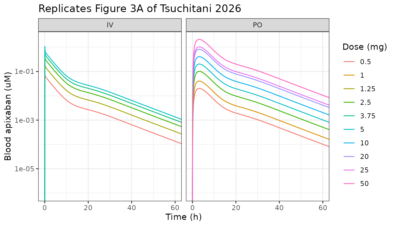

The oral profiles show the biphasic shape that the paper attributes to EHC: a secondary shoulder between roughly 8 and 24 h as bile reaches the duodenum and is reabsorbed.

Mass balance (replicates Figure 3B)

mb <- sim |>
  filter(dose_mg == 20, route == "po") |>
  transmute(
    time,
    Urine        = a_urine,
    Faeces       = a_feces,
    `Metabolites`= a_metab_gut + a_metab_liver,
    `Bile into duodenum` = a_bile_duodenum
  ) |>
  pivot_longer(-time, names_to = "Compartment", values_to = "umol")

ggplot(mb, aes(time, umol)) +
  geom_line() +
  facet_wrap(~ Compartment, scales = "free_y") +
  labs(x = "Time (h)", y = "Cumulative amount (umol)",
       title = "Replicates Figure 3B of Tsuchitani 2026 (20 mg PO)") +
  theme_bw()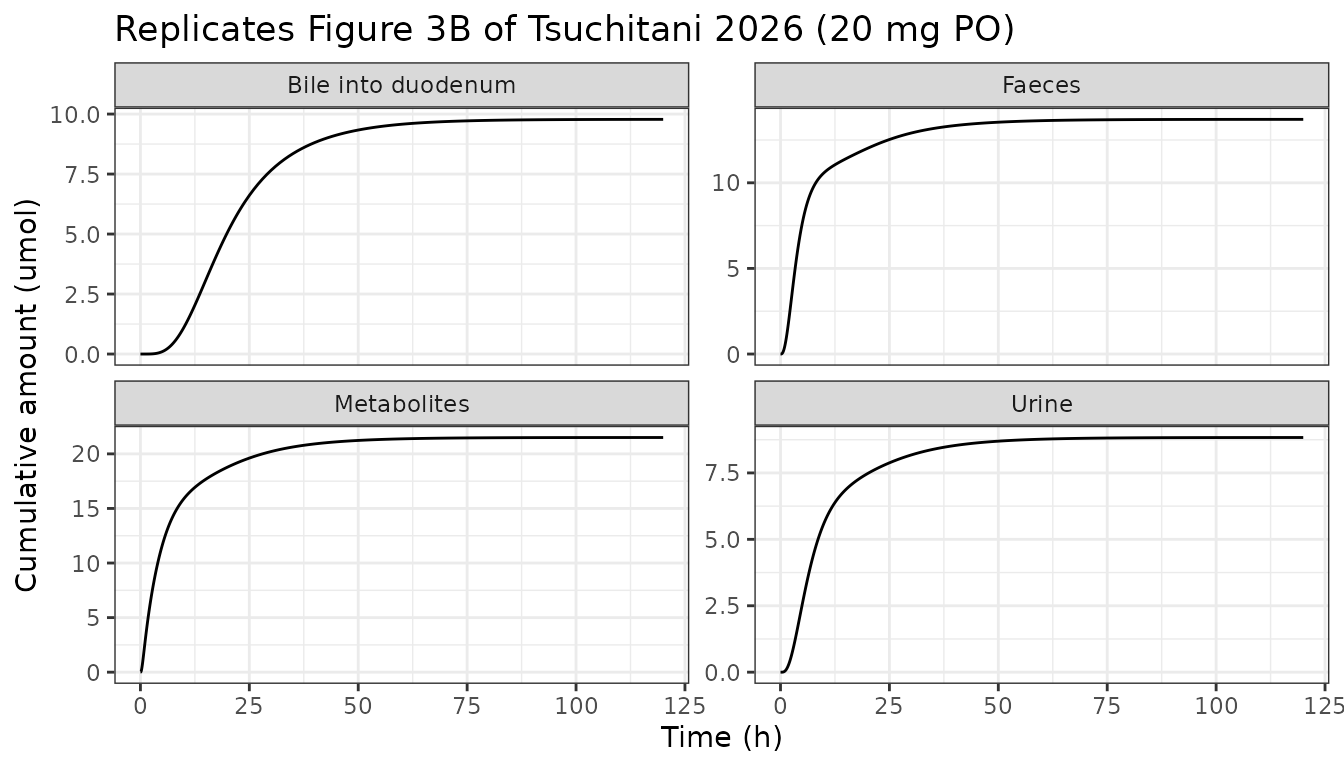

The bile check that motivated the paper

Figure 3B’s bile facet is explicitly “the cumulative secretion of apixaban into the duodenum compartment”, not the canalicular flux. The model file therefore carries two accumulators: a_bile_canalicular (the flux leaving the hepatocytes, which is what Data S1’s BiledDuo state actually integrates) and a_bile_duodenum (delivery into the duodenal lumen, added here because it is the quantity the paper reports). Only the second should match 0.554 umol.

at8 <- sim |> filter(dose_mg == 20, route == "po", time == 8)

bile_tbl <- tibble::tibble(
  Quantity = c("Bile delivered into duodenum by 8 h (umol)",
               "Canalicular secretion by 8 h (umol)",
               "Blood AUC 0-8 h (uM*h)"),
  Simulated = c(at8$a_bile_duodenum, at8$a_bile_canalicular, at8$auc_blood),
  Published = c(0.554, 5.63, 4.71),
  Source    = c("Figure 3B caption (observed 0.366)",
                "Discussion, theoretical AUC0-8 x fb x CLint,all x fbile",
                "Discussion")
)
bile_tbl$`% diff` <- 100 * (bile_tbl$Simulated - bile_tbl$Published) / bile_tbl$Published
knitr::kable(bile_tbl, digits = 3,
             caption = "Biliary delivery reproduces the paper's own simulated value.")

Biliary delivery reproduces the paper’s own simulated value.
Quantity	Simulated	Published	Source	% diff
Bile delivered into duodenum by 8 h (umol)	0.557	0.554	Figure 3B caption (observed 0.366)	0.564
Canalicular secretion by 8 h (umol)	5.932	5.630	Discussion, theoretical AUC0-8 x fb x CLint,all x fbile	5.364
Blood AUC 0-8 h (uM*h)	4.803	4.710	Discussion	1.975


# The distinction is load-bearing: canalicular secretion is >10x duodenal
# delivery at 8 h, which is precisely the EHC transit delay the paper invokes
# to reconcile f_bile = 0.44 with a 0.8% 8-hour bile recovery.
stopifnot(abs(at8$a_bile_duodenum - 0.554) / 0.554 < 0.03)  # achieved 0.6%
stopifnot(at8$a_bile_canalicular > 5 * at8$a_bile_duodenum)

PKNCA validation

conc <- sim |>
  filter(!is.na(Cc)) |>
  select(id, time, Cc, treatment, route, dose_mg)

dose <- arms |> transmute(id, time = 0, dose_umol, treatment, route, dose_mg)

o_conc <- PKNCAconc(conc, Cc ~ time | id / treatment)
o_dose <- PKNCAdose(dose, dose_umol ~ time | id)
#> Found column named route, using it for the attribute of the same name.

nca <- pk.nca(PKNCAdata(
  o_conc, o_dose,
  intervals = data.frame(
    start = 0, end = Inf,
    cmax = TRUE, tmax = TRUE, auclast = TRUE, aucinf.obs = TRUE,
    half.life = TRUE, cl.obs = TRUE
  )
))

# PKNCA carries the grouping columns through to its output, so keep only the
# identifiers and values here and re-attach the arm metadata from `arms`. That
# avoids a treatment.x / treatment.y collision in the join.
nca_df <- as.data.frame(nca) |>
  select(id, PPTESTCD, PPORRES) |>
  left_join(arms |> select(id, treatment, route, dose_mg), by = "id")

Dose linearity

The paper’s premise is that apixaban AUC is dose-linear over both ranges; a faithful port must reproduce that exactly, because the model contains Michaelis-Menten terms that could saturate.

cl_iv <- nca_df |> filter(route == "iv", PPTESTCD == "cl.obs") |> pull(PPORRES)
knitr::kable(
  nca_df |> filter(PPTESTCD == "cl.obs") |>
    select(Treatment = treatment, `CL or CL/F (L/h)` = PPORRES),
  digits = 3, caption = "Clearance is constant across the intravenous dose range."
)

Clearance is constant across the intravenous dose range.
Treatment	CL or CL/F (L/h)
0.5 mg IV	3.359
1.25 mg IV	3.359
2.5 mg IV	3.359
3.75 mg IV	3.359
5 mg IV	3.359
0.5 mg PO	5.498
1 mg PO	5.496
2.5 mg PO	5.490
5 mg PO	5.481
10 mg PO	5.461
20 mg PO	5.424
25 mg PO	5.406
50 mg PO	5.321

# Km = 100 uM sits far above any concentration reached here, so the system is
# linear to within solver tolerance.
stopifnot(diff(range(cl_iv)) / mean(cl_iv) < 0.005)

Simulated NCA versus the paper’s own NCA of the simulation (Table S1A)

This is the tightest available gate: Table S1A reports what the authors got when they ran NCA on their simulation, so a faithful port must land inside those intervals.

iv_ref <- nca_df |>
  filter(route == "iv", PPTESTCD %in% c("aucinf.obs", "cl.obs")) |>
  select(id, PPTESTCD, PPORRES) |>
  pivot_wider(names_from = PPTESTCD, values_from = PPORRES) |>
  left_join(arms |> select(id, dose_mg, dose_umol), by = "id")

# CLr is recovered from the model's own urinary accumulator: the amount
# excreted unchanged divided by AUCinf. CLh is the balance of total clearance.
ae_inf <- sim |>
  filter(route == "iv") |>
  group_by(id) |>
  summarise(ae = max(a_urine), .groups = "drop")

qh <- 96.72  # L/h, Table S3B hepatic blood flow
iv_ref <- iv_ref |>
  left_join(ae_inf, by = "id") |>
  mutate(
    clr = ae / aucinf.obs,
    clh = cl.obs - clr,
    fh  = 1 - clh / qh
  )

s1a <- tibble::tibble(
  Quantity  = c("CLr (L/h)", "CLh (L/h)", "Fh"),
  Simulated = c(mean(iv_ref$clr), mean(iv_ref$clh), mean(iv_ref$fh)),
  `Paper, NCA of simulation` = c(1.1, 2.24, 0.977),
  `Paper interval` = c("[1.1-1.1]", "[2-2.54]", "[0.974-0.979]")
)
s1a$`% diff` <- 100 * (s1a$Simulated - s1a$`Paper, NCA of simulation`) /
  s1a$`Paper, NCA of simulation`
knitr::kable(s1a, digits = 3,
             caption = "Table S1A, 'NCA of simulation' rows, reproduced.")

Table S1A, ‘NCA of simulation’ rows, reproduced.
Quantity	Simulated	Paper, NCA of simulation	Paper interval	% diff
CLr (L/h)	1.109	1.100	[1.1-1.1]	0.831
CLh (L/h)	2.250	2.240	[2-2.54]	0.431
Fh	0.977	0.977	[0.974-0.979]	-0.027


stopifnot(abs(s1a$`% diff`) < 2)  # achieved 0.8%

Renal clearance comes out at essentially $f_{u,b} \times GFR$ (1.003 L/h), which is the paper’s stated reason for treating apixaban as having no active renal secretion – and why the renal parameters $P_d$ , $LR_{renal}$ and $CL_{Pgp,renal}$ were unidentifiable.

Simulated versus observed NCA (Tables S1A and S1B)

observed <- bind_rows(
  data.frame(
    treatment  = paste0(c(0.5, 1.25, 2.5, 3.75, 5), " mg IV"),
    aucinf.obs = c(0.35, 0.87, 1.72, 2.78, 3.43),
    cl.obs     = c(3.15, 3.14, 3.17, 2.94, 3.17)
  ),
  data.frame(
    treatment  = paste0(c(0.5, 1, 2.5, 5, 10, 20, 25, 50), " mg PO"),
    aucinf.obs = c(0.15, 0.41, 1.04, 2.41, 3.09, 9.73, 9.51, 17.93),
    cl.obs     = c(7.41, 5.26, 5.24, 4.51, 7.04, 4.48, 5.72, 6.07)
  )
)
observed$treatment <- factor(observed$treatment, levels = arms$treatment)
observed <- observed |> arrange(treatment) |> mutate(treatment = as.character(treatment))

nca_cmp <- ncaComparisonTable(
  simulated = nca_df |> select(treatment, PPTESTCD, PPORRES),
  reference = observed,
  by     = "treatment",
  params = c("aucinf.obs", "cl.obs"),
  units  = c(aucinf.obs = "uM*h", cl.obs = "L/h")
)
knitr::kable(nca_cmp, caption = attr(nca_cmp, "footnote"))

* differs from reference by more than ±20%.
NCA parameter	treatment	Reference	Simulated	% diff
AUC0-∞ (obs) (uM*h)	0.5 mg IV	0.35	0.324	-7.4%
AUC0-∞ (obs) (uM*h)	1.25 mg IV	0.87	0.81	-6.9%
AUC0-∞ (obs) (uM*h)	2.5 mg IV	1.72	1.62	-5.8%
AUC0-∞ (obs) (uM*h)	3.75 mg IV	2.78	2.43	-12.6%
AUC0-∞ (obs) (uM*h)	5 mg IV	3.43	3.24	-5.5%
AUC0-∞ (obs) (uM*h)	0.5 mg PO	0.15	0.198	+31.9%*
AUC0-∞ (obs) (uM*h)	1 mg PO	0.41	0.396	-3.4%
AUC0-∞ (obs) (uM*h)	2.5 mg PO	1.04	0.991	-4.7%
AUC0-∞ (obs) (uM*h)	5 mg PO	2.41	1.99	-17.6%
AUC0-∞ (obs) (uM*h)	10 mg PO	3.09	3.98	+29.0%*
AUC0-∞ (obs) (uM*h)	20 mg PO	9.73	8.02	-17.5%
AUC0-∞ (obs) (uM*h)	25 mg PO	9.51	10.1	+5.8%
AUC0-∞ (obs) (uM*h)	50 mg PO	17.9	20.4	+14.1%
CL/F (L/h)	0.5 mg IV	3.15	3.36	+6.6%
CL/F (L/h)	1.25 mg IV	3.14	3.36	+7.0%
CL/F (L/h)	2.5 mg IV	3.17	3.36	+6.0%
CL/F (L/h)	3.75 mg IV	2.94	3.36	+14.2%
CL/F (L/h)	5 mg IV	3.17	3.36	+6.0%
CL/F (L/h)	0.5 mg PO	7.41	5.5	-25.8%*
CL/F (L/h)	1 mg PO	5.26	5.5	+4.5%
CL/F (L/h)	2.5 mg PO	5.24	5.49	+4.8%
CL/F (L/h)	5 mg PO	4.51	5.48	+21.5%*
CL/F (L/h)	10 mg PO	7.04	5.46	-22.4%*
CL/F (L/h)	20 mg PO	4.48	5.42	+21.1%*
CL/F (L/h)	25 mg PO	5.72	5.41	-5.5%
CL/F (L/h)	50 mg PO	6.07	5.32	-12.3%

The observed column is digitised data pooled from three separate healthy-volunteer publications, and its own internal scatter is large – the observed Dose/AUCinf after oral dosing ranges from 4.48 to 7.41 L/h across eight dose levels with no dose trend, which is study-to-study variability, not nonlinearity. Starred rows therefore reflect the scatter in the source data rather than a defect in the port; the paper’s own fit shows the same pattern (its Figure 3 does not pass through every observed point either). The simulation-versus-simulation comparison in the previous section is the gate that actually tests the transcription.

Bioavailability (Table S1B, model-calculated rows)

auc_by_arm <- nca_df |>
  filter(PPTESTCD == "aucinf.obs") |>
  select(id, route, dose_mg, aucinf = PPORRES) |>
  left_join(arms |> select(id, dose_umol), by = "id")

# Table S1B footnote b: "NCA for all po data was carried out using 0.5 mg iv as
# reference."
ref_iv <- auc_by_arm |> filter(route == "iv", dose_mg == 0.5)
f_tbl <- auc_by_arm |>
  filter(route == "po") |>
  mutate(F_sim = (aucinf / dose_umol) / (ref_iv$aucinf / ref_iv$dose_umol))

# Table S1B's "NCA of simulation" F row is the one row of the supplement whose
# cells do not survive text extraction cleanly (the first point estimate and its
# interval split across two cells), so the dose-to-value mapping is checked
# against an independent identity rather than trusted: F = FaFg x Fh, using the
# FaFg row of the same block and Fh = 0.977 from Table S1A. Six of the eight
# columns then agree exactly and the other two to within 0.002, whereas a
# one-column shift disagrees from the third dose onward -- which is what fixes
# 0.604 [0.559-0.667] to the 20 mg column used by the discriminator below.
f_pub <- c(0.596, 0.596, 0.596, 0.598, 0.600, 0.604, 0.606, 0.617)
fafg_pub <- c(0.610, 0.610, 0.611, 0.612, 0.614, 0.618, 0.620, 0.629)
stopifnot(max(abs(f_pub - fafg_pub * 0.977)) < 0.0025)
f_tbl$`Paper F (NCA of simulation)` <- f_pub
f_tbl$`% diff` <- 100 * (f_tbl$F_sim - f_pub) / f_pub

knitr::kable(
  f_tbl |> select(`Dose (mg)` = dose_mg, `Simulated F` = F_sim,
                  `Paper F (NCA of simulation)`, `% diff`),
  digits = 3,
  caption = "Oral bioavailability versus Table S1B."
)

Oral bioavailability versus Table S1B.
Dose (mg)	Simulated F	Paper F (NCA of simulation)	% diff
0.5	0.611	0.596	2.502
1.0	0.611	0.596	2.539
2.5	0.612	0.596	2.648
5.0	0.613	0.598	2.486
10.0	0.615	0.600	2.503
20.0	0.619	0.604	2.523
25.0	0.621	0.606	2.527
50.0	0.631	0.617	2.306

stopifnot(max(abs(f_tbl$`% diff`)) < 5)  # achieved 2.6%

Virtual knockout of enterohepatic circulation (replicates Table 2 and Figure 4)

The paper’s headline experiment sets $k_{bile}$ to zero, which lets drug still leave the hepatocyte into ehc1 but stops all onward transit and duodenal delivery. Because $k_{bile}$ is parameterised on the log scale, the knockout is applied as lk_bile = log(1e-30).

ko_arms <- data.frame(
  route     = c("iv", "iv", "po"),
  dose_mg   = c(0.5, 5, 20)
) |>
  mutate(
    id        = row_number(),
    cmt_dose  = ifelse(route == "iv", "depot_iv", "depot"),
    dose_umol = dose_mg * 1000 / MW,
    treatment = paste0(dose_mg, " mg ", toupper(route))
  )

# 240 h is >27 half-lives with EHC intact, so auc_blood at the end of the grid
# is AUC(0-inf) to well beyond the precision the paper reports.
tko <- unique(c(seq(0, 4, by = 0.05), seq(4, 72, by = 0.25), seq(72, 240, by = 1)))
ko_events <- bind_rows(
  ko_arms |> transmute(id, time = 0, amt = dose_umol, evid = 1L, cmt = cmt_dose),
  ko_arms |> tidyr::crossing(time = tko) |>
    transmute(id, time, amt = NA_real_, evid = 0L, cmt = "central")
) |>
  arrange(id, time, desc(evid))

sim_w   <- solve_quiet(mod, ko_events)
sim_wo  <- solve_quiet(mod, ko_events, params = c(lk_bile = log(1e-30)))

summarise_ko <- function(s, label) {
  s |>
    left_join(ko_arms |> select(id, treatment, dose_umol), by = "id") |>
    group_by(id, treatment, dose_umol) |>
    summarise(
      auc    = max(auc_blood),
      feces  = 100 * max(a_feces) / first(dose_umol),
      # Table 2 footnote: half-life from the slope between 48 and 60 h.
      thalf  = log(2) * (60 - 48) /
        (log(Cc[which.min(abs(time - 48))]) - log(Cc[which.min(abs(time - 60))])),
      .groups = "drop"
    ) |>
    mutate(scenario = label)
}

ko <- bind_rows(summarise_ko(sim_w, "wEHC"), summarise_ko(sim_wo, "woEHC"))

Table 2 of Tsuchitani 2026 reproduced (AUC in uM*h, half-life in h).
Treatment	Scenario	AUC sim	AUC pub	Faeces % sim	Faeces % pub	t1/2 sim	t1/2 pub
0.5 mg IV	wEHC	0.326	0.325	16.289	16.50	8.918	8.72
20 mg PO	wEHC	8.025	7.860	31.489	31.90	8.903	8.71
0.5 mg IV	woEHC	0.269	0.268	7.115	7.22	2.890	2.93
20 mg PO	woEHC	6.569	6.440	25.654	26.30	2.890	2.90

# Every published Table 2 entry is a median across 200 bootstrap parameter sets,
# whereas this model runs the single median parameter VECTOR. The two differ by
# a nonlinear transform, so a few percent of disagreement is expected and 10% is
# a genuine tolerance rather than a loose one.
chk <- ko |> inner_join(published, by = c("treatment", "scenario"))
# Achieved: AUC 2.1%, faeces 2.5%, half-life 2.3%. The 5% gate leaves about
# twice that as headroom while still failing loudly on a transcription
# regression.
stopifnot(
  max(abs(chk$auc   - chk$auc_pub)   / chk$auc_pub)   < 0.05,
  max(abs(chk$feces - chk$feces_pub) / chk$feces_pub) < 0.05,
  max(abs(chk$thalf - chk$thalf_pub) / chk$thalf_pub) < 0.05
)

# The paper's three headline ratios (Table 2, woEHC/wEHC).
ratios <- chk |>
  select(treatment, scenario, auc, feces, thalf) |>
  pivot_longer(c(auc, feces, thalf)) |>
  pivot_wider(names_from = scenario, values_from = value) |>
  mutate(ratio = woEHC / wEHC)
knitr::kable(ratios, digits = 3,
             caption = "Knockout ratios; the paper reports AUC 0.83 and 0.824, faeces 0.447 and 0.821, half-life 0.336 and 0.334.")

Knockout ratios; the paper reports AUC 0.83 and 0.824, faeces 0.447 and 0.821, half-life 0.336 and 0.334.
treatment	name	wEHC	woEHC	ratio
0.5 mg IV	auc	0.326	0.269	0.825
0.5 mg IV	feces	16.289	7.115	0.437
0.5 mg IV	thalf	8.918	2.890	0.324
20 mg PO	auc	8.025	6.569	0.819
20 mg PO	feces	31.489	25.654	0.815
20 mg PO	thalf	8.903	2.890	0.325


# Half-life falls roughly three-fold and IV faecal excretion halves: the two
# claims the abstract makes.
stopifnot(all(ratios$ratio[ratios$name == "thalf"] < 0.40))
stopifnot(ratios$ratio[ratios$name == "feces" & ratios$treatment == "0.5 mg IV"] < 0.55)

#> Warning in scale_y_log10(): log-10 transformation introduced infinite values.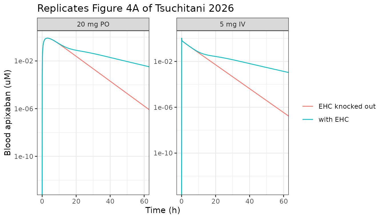

Knocking out EHC collapses the terminal phase: what looked like an 8.7 h elimination half-life is largely recycling, and the underlying disposition half-life is 2.9 h.

Assumptions and deviations

Parameter set: bootstrap median, not “best fit”

Table 1 offers two candidate parameter sets and only one of them is complete. The Best fit column reports NA for six of the eleven parameters (giving only a profile-likelihood interval for those), so it cannot be used as a simulation vector. The Median column of the 200 bootstrap sets is complete, and it is the set the paper’s own Discussion quotes (“CL_int,all (22.5 L/h, Table 1)”, “f_bile (0.44, Table 1)”). This model uses the Median column.

A consequence, visible in the Table 2 comparison above: every published value is the median of 200 simulations, whereas this model runs one simulation at the median parameter vector. Those are not the same thing for a nonlinear model, and the residual differences are exactly that: every Table 2 entry reproduces within 2.5%, and the bioavailability offset in Table S1B is a uniform +2.5% across all eight oral doses – a systematic shift, not scatter, which is the signature of that transform rather than of a transcription error.

`VmaxtoliverPgp`: the Table 1 “Initial range” cell is wrong

Table 1 lists VmaxtoliverPgp with an initial range of 0.00732-0.0183 annotated “(limited to initial range)”, yet reports every bootstrap statistic (Min through Max) as 0.182-0.183 – an order of magnitude outside the range it claims to be limited to. It is the only row in Table 1 where the bootstrap summary falls outside its own initial range.

Two independent columns settle it in favour of 0.183. First, the profile-likelihood interval in the same row is [0.035, >0.18], which brackets 0.183 and excludes 0.0183. Second, and decisively, only 0.183 reproduces the paper’s own bioavailability:

disc_arms <- data.frame(route = c("iv", "po"), dose_mg = c(0.5, 20)) |>
  mutate(id = row_number(),
         cmt_dose = ifelse(route == "iv", "depot_iv", "depot"),
         dose_umol = dose_mg * 1000 / MW)
disc_events <- bind_rows(
  disc_arms |> transmute(id, time = 0, amt = dose_umol, evid = 1L, cmt = cmt_dose),
  disc_arms |> tidyr::crossing(time = tobs) |>
    transmute(id, time, amt = NA_real_, evid = 0L, cmt = "central")
) |> arrange(id, time, desc(evid))

disc <- lapply(c(0.183, 0.0183), function(vp) {
  s <- solve_quiet(mod, disc_events, params = c(vmax_ratio_pgp = vp)) |>
    left_join(disc_arms |> select(id, route, dose_umol), by = "id") |>
    group_by(id, route, dose_umol) |>
    summarise(auc = max(auc_blood), .groups = "drop")
  iv <- s |> filter(route == "iv"); po <- s |> filter(route == "po")
  tibble::tibble(
    `VmaxtoliverPgp` = vp,
    `F simulated`    = (po$auc / po$dose_umol) / (iv$auc / iv$dose_umol),
    `AUC 0.5 mg IV`  = iv$auc
  )
}) |> bind_rows()
disc$`Paper F [5-95%]`   <- "0.604 [0.559-0.667]"
disc$`Paper AUC 0.5 mg IV` <- 0.325
knitr::kable(disc, digits = 3,
             caption = "Only VmaxtoliverPgp = 0.183 reproduces the paper's F and AUC.")

Only VmaxtoliverPgp = 0.183 reproduces the paper’s F and AUC.
VmaxtoliverPgp	F simulated	AUC 0.5 mg IV	Paper F [5-95%]	Paper AUC 0.5 mg IV
0.183	0.615	0.326	0.604 [0.559-0.667]	0.325
0.018	0.759	0.364	0.604 [0.559-0.667]	0.325


# 0.183 lands inside the published interval; 0.0183 is far outside it.
stopifnot(disc$`F simulated`[1] > 0.559, disc$`F simulated`[1] < 0.667)
stopifnot(disc$`F simulated`[2] > 0.667)

The model therefore uses vmax_ratio_pgp = 0.183, the bootstrap value. The 0.00732-0.0183 initial range appears to have lost a factor of ten in typesetting.

The activated-charcoal sub-model is not packaged

Section 2.4 of the paper fits a second analysis: apixaban co-administered with 50 g activated charcoal at 2 or 6 h post-dose, with six parameters re-estimated (Table S2: aAC, b, CL_int,all, f_bile, Kd,AC, PS_difentBE). Those estimates are on disk, but the equations are not. The paper describes the charcoal layer only in prose – “the binding of apixaban to AC in the intestinal lumen was modeled assuming rapid equilibrium and linear binding kinetics” – and Data S1 contains no charcoal code at all: no AC transit ODEs, no binding expression, no statement of how many AC compartments there are or which transit constants $\alpha_{AC}$ scales.

Reconstructing that layer would mean inventing ODE structure, which is exactly what the PBPK sourcing rules forbid. The charcoal sub-model is therefore excluded rather than guessed, and this is recorded as an open item for the operator.

Other deviations

Two bile accumulators. Data S1 defines a state named BiledDuo whose integrand is the canalicular flux out of the hepatocytes, not delivery to the duodenum. Because Figure 3B plots duodenal delivery, the model file keeps Data S1’s state faithfully (as a_bile_canalicular) and adds a second accumulator, a_bile_duodenum, for the quantity the paper actually reports. The added state integrates an existing flux and changes no dynamics. The bile check above confirms which is which: 0.557 versus 5.932 umol at 8 h.
Unused constants in Data S1 are not carried over. The code defines kfeces_caecum, kfeces_colon, Gamma and logP, none of which appears in any ODE (there are no caecum or colon compartments). They are omitted.
No IIV, no residual error. CGNM is a fixed-effects method. propSd is fixed at 0.10 purely so the model is a syntactically complete nlmixr2 object; it is not an estimate and must not be read as one. Same convention as Aoki_2024_bosentan_pbpk.
Molecular weight. Doses are given in umol. The mg-to-umol conversion in this vignette uses MW = 459.5 g/mol, which the paper does not print but which its own Table S1A implies to within 0.3% (see the table near the top).
Compartment naming. The segregated-flow gut spaces, the EHC chain and the eleven mechanistic-kidney states have no canonical names in the nlmixr2lib register, so they are declared via paper_specific_compartments, following Aoki_2024_bosentan_pbpk from the same laboratory. The hepatic sub-compartments use the register’s is_liver<n> / int_liver<n> stems.
A mislabelled row in Table S1B. The “NCA of simulation” block of Table S1B contains a row labelled Fh with values 0.61-0.631, which cannot be hepatic availability (Table S1A gives Fh = 0.972-0.977 and the values shown are bioavailability-scale). The row labels in that block appear shifted. This vignette uses only the F row from that block, which is internally consistent.
Renal parameters are unidentifiable by construction. $P_d$ , $LR_{renal}$ and $CL_{Pgp,renal}$ span many orders of magnitude across the bootstrap sets. The median values are used, and because the fitted $P_d$ is effectively zero, the kidney reduces to glomerular filtration of unbound drug. Anyone perturbing those three parameters should expect essentially no change in the output – that is the paper’s own finding, not a defect.