Caspofungin (Wu 2022)

Model and source

• Citation: Wu Z, Lan J, Wang X, Wu Y, Yao F, Wang Y, Zhao B, Wang Y, Chen J, Chen C. Population pharmacokinetics of caspofungin and dose simulations in heart transplant recipients. Antimicrob Agents Chemother. 2022;66(5):e02249-21. doi:10.1128/aac.02249-21. PMC9116478.
• Description: Two-compartment population PK model for intravenous caspofungin in critically ill adults after cardiac surgery, pooling heart transplant recipients and non-transplant cardiac-surgery patients (Wu 2022). Serum albumin enters as a power covariate (centred at 37.42 g/L) on clearance; heart transplantation, ECMO and CRRT were screened and not retained. Exponential IIV on CL, Vc and Vp (Q IIV fixed to 0); residual error is the linear sum of an additive and a proportional SD. NONMEM 7.3 FOCE-I; 58 patients, 414 samples.
• Article: https://doi.org/10.1128/aac.02249-21
• Open-access full text: https://www.ncbi.nlm.nih.gov/pmc/articles/PMC9116478/

Wu 2022 studied caspofungin in critically ill adults in a surgical ICU after cardiac surgery. Twenty-seven had received a heart transplant and 31 had had other cardiac surgery. Heart transplantation did not affect caspofungin PK once serum albumin was accounted for: the final two-compartment model keeps only albumin, as a power covariate on clearance. Lower albumin gives a higher clearance, which the authors attribute to a larger unbound fraction of this highly protein-bound drug.

Population

Fifty-eight patients at one centre in Guangzhou, China (July 2019 - July 2021), gave 414 plasma samples (Results and Table 1). The heart-transplant group had a median age of 50 years, weight 59.5 kg, 19% women and a median albumin of 40.3 g/L (29.7-49.3). The control group had a median age of 58 years, weight 62.0 kg, 32% women and a median albumin of 33.7 g/L (26.41-48.40). About half of each group was on CRRT and about a quarter on ECMO; the median SOFA score was 9-10. Every patient received a 70 mg loading dose and then 50 mg every 24 h as a 1-h intravenous infusion. Samples were taken before the dose and 1, 2, 6, 10, 16 and 24 h after it, on at least 3 days.

Source trace

The supplementary material prints the NONMEM control stream. Its $THETA and $OMEGA values agree with Table 2, and it supplies the albumin centring value (37.42 g/L) that the main text does not print.

Model element	Value	Source location
Two-compartment model, IV infusion (ADVAN3 TRANS4)	–	Results; supplementary control stream $SUBROUTINES
lcl (CL at ALB = 37.42 g/L)	0.385 L/h	Table 2; control stream THETA(1)
lvc (Vc)	4.27 L	Table 2; THETA(2)
lq (Q)	2.85 L/h	Table 2; THETA(3)
lvp (Vp)	6.01 L	Table 2; THETA(4)
e_alb_cl	-1.01	Table 2, ‘theta ALB-CL’; THETA(7)
etalcl	0.112 (33.5%)	Table 2; control stream $OMEGA
etalvc	0.455 (67.5%)	Table 2; $OMEGA
etalq	0 FIX	Table 2; $OMEGA
etalvp	0.2275 (47.7%)	Table 2 ($OMEGA prints 0.22)
propSd	0.134	Table 2; THETA(5)
addSd	0.213 mg/L	Table 2; THETA(6)
CL = THETA(1) exp(ETA(1)) (ALB/37.42)^THETA(7)	–	Control stream $PK; Methods equation 2
W = IPRED THETA(5) + THETA(6), $SIGMA 1 FIX	–	Control stream $ERROR
70 mg loading, then 50 mg q24h, 1-h infusion	–	Methods, ‘Blood sample collection’
PTA: AUC = Dose / CL; AUC/MIC targets 865, 450, 1185	–	Methods, ‘Simulations’; supplementary Matlab code

Virtual cohort

Each group has 100 subjects. Albumin is drawn log-normally around each group’s Table 1 median, with a log-scale SD of one quarter of the log range, and is truncated to the observed range. Albumin is held constant within a subject.

set.seed(2022)
rxode2::rxSetSeed(2022)
n_arm <- 100

draw_alb <- function(n, med, lo, hi) {
  sdl <- log(hi / lo) / 4
  out <- numeric(0)
  while (length(out) < n) {
    x <- exp(rnorm(n, log(med), sdl))
    out <- c(out, x[x >= lo & x <= hi])
  }
  out[seq_len(n)]
}

subj <- dplyr::bind_rows(
  data.frame(id = seq_len(n_arm), group = "Heart transplant", ALB = draw_alb(n_arm, 40.3, 29.7, 49.3)),
  data.frame(id = n_arm + seq_len(n_arm), group = "Control", ALB = draw_alb(n_arm, 33.7, 26.41, 48.40))
)
subj |>
  dplyr::group_by(group) |>
  dplyr::summarise(median_ALB = median(ALB), min_ALB = min(ALB), max_ALB = max(ALB), .groups = "drop") |>
  dplyr::rename("Group" = group, "Median ALB (g/L)" = median_ALB, "Min" = min_ALB, "Max" = max_ALB) |>
  knitr::kable(digits = 1, caption = "Virtual cohort albumin.")

Virtual cohort albumin.

Group	Median ALB (g/L)	Min	Max
Control	34.2	26.8	44.8
Heart transplant	41.1	30.5	48.6

inf_dur <- 1
dose_times <- seq(0, 96, by = 24)
dose_amts <- c(70, rep(50, length(dose_times) - 1))
obs_times <- sort(unique(c(seq(0, 120, by = 0.5), dose_times + 1)))

make_events <- function(s) {
  dose <- data.frame(
    id = s$id, time = dose_times, evid = 1, amt = dose_amts,
    rate = dose_amts / inf_dur, cmt = "central"
  )
  obs <- data.frame(id = s$id, time = obs_times, evid = 0, amt = 0, rate = 0, cmt = "central")
  ev <- rbind(dose, obs)
  ev$ALB <- s$ALB
  ev$group <- s$group
  ev[order(ev$time, -ev$evid), ]
}
events <- do.call(rbind, lapply(split(subj, subj$id), make_events))

Simulation

mod <- readModelDb("Wu_2022_caspofungin")
sim <- rxode2::rxSolve(mod, events, keep = c("group"), returnType = "data.frame")
#> ℹ parameter labels from comments will be replaced by 'label()'
#> ℹ omega/sigma items treated as zero: 'etalq'

Concentration-time profiles

The paper’s VPC (Figure 3) overlays observed data, which are not available. The plot below shows the simulated median and 5th-95th percentiles over the first five days for each group.

sim |>
  dplyr::group_by(group, time) |>
  dplyr::summarise(
    med = median(Cc), lo = quantile(Cc, 0.05), hi = quantile(Cc, 0.95),
    .groups = "drop"
  ) |>
  ggplot(aes(time, med, colour = group, fill = group)) +
  geom_ribbon(aes(ymin = lo, ymax = hi), alpha = 0.15, colour = NA) +
  geom_line() +
  labs(
    x = "Time after first dose (h)", y = "Caspofungin (mg/L)", colour = NULL, fill = NULL,
    caption = "Simulated 70 mg loading dose, then 50 mg q24h (1-h infusion)."
  ) +
  theme_bw()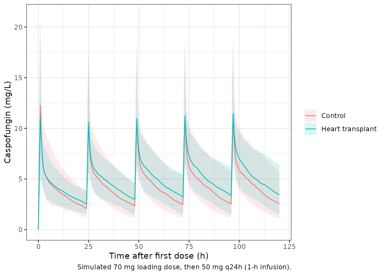

PKNCA validation

Table 3 does not say which dosing day its Cmax, Cmin and AUC describe. The third dose (48-72 h), the last of the minimum three sampling days, is used.

conc <- sim |>
  dplyr::filter(!is.na(Cc)) |>
  dplyr::select(id, time, Cc, group)
dose <- events |>
  dplyr::filter(evid == 1) |>
  dplyr::select(id, time, amt, group)
conc_obj <- PKNCA::PKNCAconc(conc, Cc ~ time | group + id, concu = "mg/L", timeu = "h")
dose_obj <- PKNCA::PKNCAdose(dose, amt ~ time | group + id, doseu = "mg")
intervals <- data.frame(start = 48, end = 72, cmax = TRUE, cmin = TRUE, auclast = TRUE)
nca_res <- as.data.frame(PKNCA::pk.nca(PKNCA::PKNCAdata(conc_obj, dose_obj, intervals = intervals))$result)

nca_res |>
  dplyr::filter(PPTESTCD %in% c("cmax", "cmin", "auclast")) |>
  dplyr::group_by(group, PPTESTCD) |>
  dplyr::summarise(
    median = median(PPORRES), q05 = quantile(PPORRES, 0.05),
    q95 = quantile(PPORRES, 0.95), .groups = "drop"
  ) |>
  dplyr::mutate(parameter = nlmixr2lib::ncaParamLabel(PPTESTCD)) |>
  dplyr::select(group, parameter, median, q05, q95) |>
  dplyr::rename(
    "Group" = group, "NCA parameter" = parameter, "Median" = median,
    "5th percentile" = q05, "95th percentile" = q95
  ) |>
  knitr::kable(digits = 2, caption = "Simulated NCA of the third dose (Cmax, Cmin in mg/L; AUC in mg.h/L).")

Simulated NCA of the third dose (Cmax, Cmin in mg/L; AUC in mg.h/L).

Group	NCA parameter	Median	5th percentile	95th percentile
Control	AUClast	105.71	67.50	178.86
Control	Cmax	10.89	6.25	18.28
Control	Cmin	2.35	1.13	4.53
Heart transplant	AUClast	125.82	76.82	181.48
Heart transplant	Cmax	11.00	6.38	18.59
Heart transplant	Cmin	2.99	1.49	4.70

Comparison against the published values (Table 3)

published <- data.frame(
  group = c("Heart transplant", "Control"),
  cmax = c(11.74, 7.89),
  cmin = c(3.59, 2.92),
  auclast = c(126.86, 105.64)
)
cmp <- nlmixr2lib::ncaComparisonTable(
  simulated = nca_res,
  reference = published,
  by = "group",
  params = c("cmax", "cmin", "auclast"),
  units = c(cmax = "mg/L", cmin = "mg/L", auclast = "mg*h/L"),
  tolerance_pct = 20
)
knitr::kable(cmp, caption = "Simulated vs published medians (Wu 2022 Table 3). * differs by >20%.")

Simulated vs published medians (Wu 2022 Table 3). * differs by >20%.

NCA parameter	group	Reference	Simulated	% diff
Cmax (mg/L)	Heart transplant	11.7	11	-6.3%
Cmax (mg/L)	Control	7.89	10.9	+38.0%*
Cmin (mg/L)	Heart transplant	3.59	2.99	-16.8%
Cmin (mg/L)	Control	2.92	2.35	-19.6%
AUClast (mg*h/L)	Heart transplant	127	126	-0.8%
AUClast (mg*h/L)	Control	106	106	+0.1%

attr(cmp, "footnote")
#> [1] "* differs from reference by more than ±20%."

# Centre-of-distribution check (one value per simulated subject, so assert on
# the median only): AUC is set by CL and its albumin covariate.
auc_med <- nca_res |>
  dplyr::filter(PPTESTCD == "auclast") |>
  dplyr::group_by(group) |>
  dplyr::summarise(auc = median(PPORRES), .groups = "drop") |>
  dplyr::left_join(published[, c("group", "auclast")], by = "group")
stopifnot(all(abs(auc_med$auc / auc_med$auclast - 1) < 0.12))

The AUC matches Table 3 in both groups. The higher albumin of the heart-transplant group lowers its clearance in the model, which reproduces that group’s higher AUC. The simulated Cmin is 17-20% below Table 3 in both groups. Cmax is the weak point: the heart-transplant Cmax matches, but the control Cmax is about 38% too high. Table 3 reports individual Vc medians of 3.14 L in the heart-transplant group and 5.27 L in the control group. The model has no covariate on Vc, so both groups share the 4.27 L typical value, and the simulated Cmax hardly differs between groups. Table 3 summarises individual (post hoc) estimates, so this group difference sits inside the model’s 67.5% IIV on Vc rather than in its fixed effects.

Replicate Figure 4 (probability of target attainment)

The paper computes PTA from the steady-state AUC over 24 h, AUC = Dose / CL, with clearance log-normal across subjects (Methods, ‘Simulations’). The values below use the model’s typical clearance at the 37 g/L albumin of Figure 4 and its CL IIV. The AUC/MIC targets are 865 (C. albicans), 450 (C. glabrata) and 1185 (C. parapsilosis).

First, the PKNCA steady-state AUC from a typical-value solve is checked against Dose / CL, which the PTA calculation relies on.

typ_ev <- rxode2::et(amt = 50, rate = 50 / inf_dur, ii = 24, addl = 19, cmt = "central") |>
  rxode2::et(seq(0, 480, by = 0.1)) |>
  as.data.frame()
typ_ev$ALB <- 37
typ_ev$id <- 1L
typ <- rxode2::rxSolve(rxode2::zeroRe(mod), typ_ev, returnType = "data.frame")
#> ℹ parameter labels from comments will be replaced by 'label()'
#> ℹ omega/sigma items treated as zero: 'etalcl', 'etalvc', 'etalq', 'etalvp'
typ$id <- 1L
cl_typ <- typ$cl[1]

ss_nca <- as.data.frame(PKNCA::pk.nca(PKNCA::PKNCAdata(
  PKNCA::PKNCAconc(typ[, c("id", "time", "Cc")], Cc ~ time | id),
  PKNCA::PKNCAdose(typ_ev[typ_ev$evid == 1, c("id", "time", "amt")], amt ~ time | id),
  intervals = data.frame(start = 456, end = 480, auclast = TRUE)
))$result)
auc_tau <- ss_nca$PPORRES[ss_nca$PPTESTCD == "auclast"]
c(cl_typical = cl_typ, auc_tau = auc_tau, dose_over_cl = 50 / cl_typ)
#>   cl_typical      auc_tau dose_over_cl 
#>    0.3894142  128.3967616  128.3979811
# Same drawn parameters on both sides (no IIV): pure numerical error.
stopifnot(
  abs(cl_typ - 0.385 * (37 / 37.42)^-1.01) < 1e-8,
  abs(auc_tau * cl_typ / 50 - 1) < 0.005
)

omega_cl <- sqrt(0.112)
targets <- c("C. albicans" = 865, "C. glabrata" = 450, "C. parapsilosis" = 1185)
pta_grid <- tidyr::expand_grid(
  species = names(targets),
  dose = c(50, 70, 100, 150, 200),
  mic = c(0.03, 0.06, 0.125, 0.25, 0.5, 1)
) |>
  dplyr::mutate(
    target = targets[species],
    pta = pnorm((log(dose / (mic * target)) - log(cl_typ)) / omega_cl)
  )

ggplot(pta_grid, aes(mic, pta, colour = factor(dose))) +
  geom_line() +
  geom_point() +
  facet_wrap(~species, ncol = 1) +
  labs(
    x = "MIC (mg/L)", y = "PTA", colour = "Dose (mg)",
    caption = "Replicates Figure 4 of Wu 2022 (median lines; ALB = 37 g/L)."
  ) +
  theme_bw()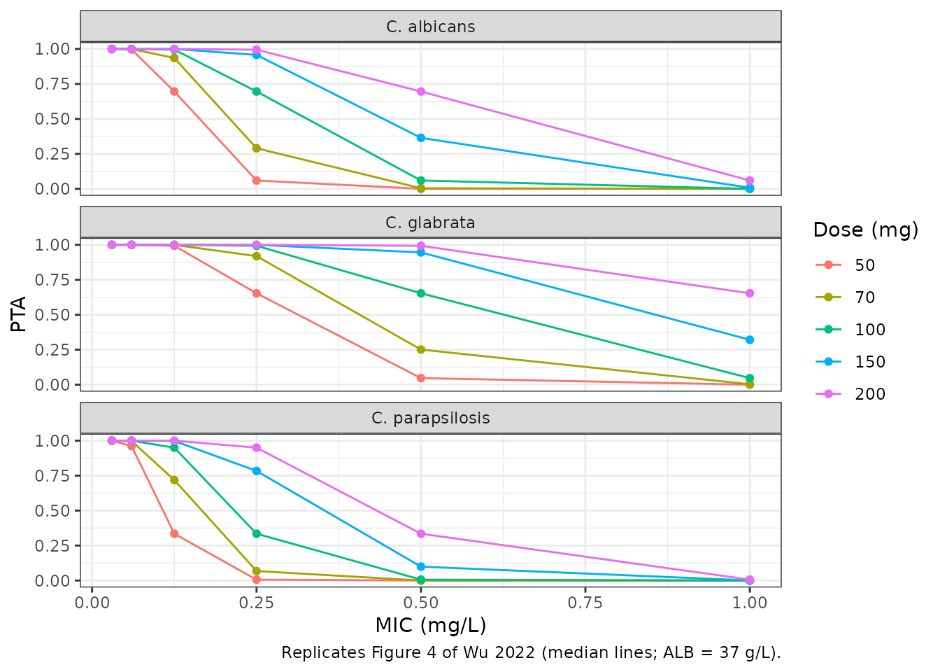

The maintainers read the median PTA lines of Figure 4 at points where the lines are steep, so a parameter error would show:

fig4 <- data.frame(
  species = c(rep("C. albicans", 5), rep("C. glabrata", 5), rep("C. parapsilosis", 5)),
  dose = c(50, 70, 100, 150, 200, 50, 70, 100, 150, 200, 50, 70, 100, 150, 200),
  mic = c(0.125, 0.25, 0.25, 0.5, 0.5, 0.25, 0.5, 0.5, 1, 1, 0.125, 0.125, 0.25, 0.25, 0.5),
  pta_fig4 = c(0.70, 0.29, 0.71, 0.37, 0.71, 0.67, 0.24, 0.66, 0.32, 0.67, 0.33, 0.74, 0.33, 0.80, 0.33)
)
fig4_cmp <- dplyr::left_join(fig4, pta_grid, by = c("species", "dose", "mic")) |>
  dplyr::mutate(diff = pta - pta_fig4)
fig4_cmp |>
  dplyr::select(species, dose, mic, pta_fig4, pta, diff) |>
  dplyr::rename(
    "Species" = species, "Dose (mg)" = dose, "MIC (mg/L)" = mic,
    "PTA, Figure 4 (read)" = pta_fig4, "PTA, model" = pta, "Difference" = diff
  ) |>
  knitr::kable(digits = 2, caption = "Model PTA against values read from Figure 4.")

Model PTA against values read from Figure 4.

Species	Dose (mg)	MIC (mg/L)	PTA, Figure 4 (read)	PTA, model	Difference
C. albicans	50	0.12	0.70	0.70	0.00
C. albicans	70	0.25	0.29	0.29	0.00
C. albicans	100	0.25	0.71	0.70	-0.01
C. albicans	150	0.50	0.37	0.36	-0.01
C. albicans	200	0.50	0.71	0.70	-0.01
C. glabrata	50	0.25	0.67	0.65	-0.02
C. glabrata	70	0.50	0.24	0.25	0.01
C. glabrata	100	0.50	0.66	0.65	-0.01
C. glabrata	150	1.00	0.32	0.32	0.00
C. glabrata	200	1.00	0.67	0.65	-0.02
C. parapsilosis	50	0.12	0.33	0.33	0.00
C. parapsilosis	70	0.12	0.74	0.72	-0.02
C. parapsilosis	100	0.25	0.33	0.33	0.00
C. parapsilosis	150	0.25	0.80	0.78	-0.02
C. parapsilosis	200	0.50	0.33	0.33	0.00

# Deterministic (no random draws). The tolerance covers reading the figure
# and the paper's use of bootstrap-median parameters in its Matlab code.
stopifnot(max(abs(fig4_cmp$diff)) < 0.06)

The model reproduces Figure 4 to within the precision of reading the figure.

Albumin dependence (Figure S1)

Figure S1 repeats Figure 4 at other albumin levels. Because CL scales as (ALB / 37.42)^-1.01, the AUC scales almost in proportion to albumin. The table gives the 50 mg dose’s PTA against C. albicans.

alb_tab <- tidyr::expand_grid(ALB = c(25, 30, 37, 45, 50), mic = c(0.06, 0.125, 0.25)) |>
  dplyr::mutate(
    cl = 0.385 * (ALB / 37.42)^-1.01,
    pta = pnorm((log(50 / (mic * 865)) - log(cl)) / omega_cl)
  )
alb_tab |>
  dplyr::select(ALB, mic, pta) |>
  tidyr::pivot_wider(names_from = mic, values_from = pta, names_prefix = "MIC ") |>
  dplyr::rename("ALB (g/L)" = ALB) |>
  knitr::kable(digits = 2, caption = "PTA, 50 mg q24h, C. albicans (AUC/MIC > 865).")

PTA, 50 mg q24h, C. albicans (AUC/MIC > 865).

ALB (g/L)	MIC 0.06	MIC 0.125	MIC 0.25
25	0.94	0.25	0.00
30	0.98	0.45	0.01
37	1.00	0.70	0.06
45	1.00	0.87	0.17
50	1.00	0.92	0.26

Structural checks

The albumin covariate equation is checked against hand calculation.

one <- function(alb) {
  e <- data.frame(id = 1L, time = c(0, 1), evid = c(1, 0), amt = c(50, 0), cmt = "central", ALB = alb)
  r <- rxode2::rxSolve(rxode2::zeroRe(mod), e, returnType = "data.frame")
  r[1, c("cl", "vc", "q", "vp")]
}
m25 <- one(25)
#> ℹ parameter labels from comments will be replaced by 'label()'
#> ℹ omega/sigma items treated as zero: 'etalcl', 'etalvc', 'etalq', 'etalvp'
m3742 <- one(37.42)
#> ℹ parameter labels from comments will be replaced by 'label()'
#> ℹ omega/sigma items treated as zero: 'etalcl', 'etalvc', 'etalq', 'etalvp'
stopifnot(
  abs(m3742$cl - 0.385) < 1e-8, abs(m3742$vc - 4.27) < 1e-8,
  abs(m3742$q - 2.85) < 1e-8, abs(m3742$vp - 6.01) < 1e-8,
  abs(m25$cl - 0.385 * (25 / 37.42)^-1.01) < 1e-8
)

Assumptions and deviations

• Albumin centring. The Methods describe continuous covariates as (cov / cov_ave)^theta without printing the average. The supplementary control stream and Matlab code both use 37.42 g/L, which is used here. The Methods call 37 g/L the median, and Figure 4 is drawn at 37 g/L.
• IIV scale. Table 2 reports IIV in percent. The control stream $OMEGA values (0.112, 0.455, 0.22) are the squares of the Table 2 percentages divided by 100, so the percentages are sqrt(omega^2). The Vp variance uses the more precise Table 2 value, 0.477^2 = 0.2275. The paper’s Matlab code instead converts the bootstrap CL percentage as a CV, sqrt(log(CV^2 + 1)); the difference is small (0.319 against 0.335) and Figure 4 is reproduced either way.
• IIV on Q. Fixed to zero in the final model (Table 2, $OMEGA 0 FIX), kept as etalq ~ fixed(0).
• Residual error. The control stream sets the residual SD to IPRED x 0.134 + 0.213 (a linear sum, $SIGMA 1 FIX), encoded with combined1().
• Time-varying albumin. Albumin was recorded on each sampling day. The virtual cohort holds it constant within a subject; the model accepts a time-varying column.
• Table 3 comparison. The paper does not say which dosing day Table 3 describes. The third dose is used. Table 3’s group difference in Cmax is not explained by the model’s covariates, so the control-group Cmax is overpredicted (see the comparison above).
• Figure 4. The paper’s Matlab code samples bootstrap uncertainty and plots the median PTA across 1000 draws. The replication uses the final estimates without parameter uncertainty, which gives the median lines but not the shaded intervals.