N,N-dimethyltryptamine EEG response (Eckernas 2023)
Source:vignettes/articles/Eckernas_2023_dimethyltryptamine_EEG.Rmd
Eckernas_2023_dimethyltryptamine_EEG.RmdModel and source
Eckernas et al. (2023) linked plasma N,N-dimethyltryptamine (DMT)
concentrations to three electroencephalography (EEG) readouts –
alpha-band power, beta-band power and the Lempel-Ziv complexity (LZc)
score of signal diversity. The three readouts were fitted as three
separate NONMEM runs (Appendix S1 contains one
$PROBLEM per readout), each an effect-compartment model
sitting on the same plasma PK model whose parameters were fixed from the
authors’ earlier population PK analysis. Following the library
convention of replicating the authors’ structure, the paper contributes
three model files that share this vignette.
modAlpha <- readModelDb("Eckernas_2023_dimethyltryptamine_alphaPower")
modBeta  <- readModelDb("Eckernas_2023_dimethyltryptamine_betaPower")
modLZc <- readModelDb("Eckernas_2023_dimethyltryptamine_LZc")- Citation: Eckernas E, Timmermann C, Carhart-Harris R, Roshammar D, Ashton M. N,N-dimethyltryptamine affects electroencephalography response in a concentration-dependent manner - A pharmacokinetic/pharmacodynamic analysis. CPT Pharmacometrics Syst Pharmacol. 2023;12(4):474-486. doi:10.1002/psp4.12933. The plasma PK parameters are fixed from Eckernas E, Timmermann C, Carhart-Harris R, Roshammar D, Ashton M. Population pharmacokinetic/pharmacodynamic modelling of the psychedelic experience induced by N,N-dimethyltryptamine - implications for dose considerations. Clin Transl Sci. 2022;15(12):2928-2937; those fixed values are reproduced in Table S1 of the 2023 paper and in its Appendix S1 NONMEM control streams.
- Article: https://doi.org/10.1002/psp4.12933
- Supplement (Table S1, Appendix S1 NONMEM control streams): https://doi.org/10.1002/psp4.12933 (Supporting Information)
Descriptions:
- Alpha power – Effect-compartment sigmoidal Imax PK/PD model for the suppression of EEG alpha power by intravenous N,N-dimethyltryptamine (DMT) in healthy adults (Eckernas 2023). Plasma DMT is described by a two-compartment model with first-order elimination from the central compartment whose parameters are fixed from the upstream population PK analysis (Eckernas 2022, reproduced in Table S1). Alpha power is driven by the effect-site (biophase) concentration through a sigmoidal Imax function with Imax fixed to 1, i.e. DMT is able to fully suppress alpha power. Between-subject variability is on baseline alpha power (with a negatively skewed Box-Cox transformation of the eta) and on the effect-site IC50; between-occasion variability is on baseline alpha power. Residual variability on alpha power is proportional.
- Beta power – Effect-compartment sigmoidal Imax PK/PD model for the suppression of EEG beta power by intravenous N,N-dimethyltryptamine (DMT) in healthy adults (Eckernas 2023). Plasma DMT is described by a two-compartment model with first-order elimination from the central compartment whose parameters are fixed from the upstream population PK analysis (Eckernas 2022, reproduced in Table S1). Beta power is driven by the effect-site (biophase) concentration through a sigmoidal Imax function; unlike alpha power, suppression is only partial, with Imax estimated at 0.70. Between-subject variability is on baseline beta power and on the effect-site IC50 as a correlated block; between-occasion variability is on baseline beta power. Residual variability on beta power is proportional.
- LZc score – Effect-compartment sigmoidal Emax PK/PD model for the increase in EEG signal diversity, measured as the Lempel-Ziv complexity (LZc) score, produced by intravenous N,N-dimethyltryptamine (DMT) in healthy adults (Eckernas 2023). Plasma DMT is described by a two-compartment model with first-order elimination from the central compartment whose parameters are fixed from the upstream population PK analysis (Eckernas 2022, reproduced in Table S1). The LZc score is driven by the effect-site (biophase) concentration through a sigmoidal Emax function with a maximum relative increase of about 10% over baseline. Between-subject variability is on baseline LZc, on the effect-site EC50 and on Emax; between-occasion variability is on baseline LZc. Residual variability on the LZc score is additive.
Population
Data came from a single-blind, placebo-controlled, fixed-sequence pilot study run at the National Institute of Health Research Imperial Clinical Research Facility (London, UK). Thirteen healthy volunteers (seven men; median age 33 years, range 22-48) received placebo at their first visit and a single intravenous bolus of DMT fumarate at their second visit one week later. Doses were escalated across participants to find a level producing the intended psychedelic intensity: 7 mg (n = 3), 14 mg (n = 4), 18 mg (n = 1) and 20 mg (n = 5). Nine plasma samples per subject per occasion were collected over 60 minutes and assayed by LC-MS/MS.
EEG was recorded with a 32-channel Brainproducts system at 1000 Hz, band-pass filtered at 1-45 Hz, averaged across channels and summarised as one mean value per minute for modelling. EEG from one 20 mg participant was excluded for excessive movement artifacts, so the PD models were fitted to 12 participants (252 post-DMT and 238 post-placebo EEG observations per readout). Only alpha power, beta power and LZc showed a visually apparent exposure-response relationship and were carried forward; delta and theta power were not. No covariate effects were explored, because of the small sample size.
The same information is available programmatically via
readModelDb("Eckernas_2023_dimethyltryptamine_alphaPower")()$population.
Dose units and the molar conversion
The models work in molar units: doses are amounts in
nmol, so Cc = central / vc is in nmol/L (= nM), which is
the unit in which the paper reports IC50,e and EC50,e. The paper states
doses only as milligrams of DMT fumarate and never gives the salt
molecular weight or the molar conversion it used, so the conversion
below was digitised from Figure 5.
In Figure 5 the simulated 20 mg plasma concentration axis spans 0 to
285 nM (the panel’s data range, recovered from the axis tick calibration
and ggplot’s 5% axis expansion). With the fixed Vc = 221 L
and an intravenous bolus, C0 = Dose / Vc, so 20 mg
corresponds to 285.4 * 221 = 63.1 umol, i.e. about
3150 nmol per mg of DMT fumarate (an implied salt
molecular weight of about 317 g/mol). That single figure-derived
constant is used for every dose in this vignette and is cross-checked
three independent ways below.
nmolPerMg <- 3150  # figure-derived; see text above and "Assumptions and deviations"
doseMg    <- c(1, 4, 7, 10, 14, 20)          # Eckernas 2023 Figure 4 simulation dose levels
doseNmol  <- doseMg * nmolPerMg
data.frame(
  `Dose (mg DMT fumarate)` = doseMg,
  `Dose (nmol)`            = doseNmol,
  `C0 = Dose / Vc (nM)`    = round(doseNmol / 221, 1),
  check.names = FALSE
) |>
knitr::kable(caption = "Molar dose conversion used throughout this vignette.")| Dose (mg DMT fumarate) | Dose (nmol) | C0 = Dose / Vc (nM) |
|---|---|---|
| 1 | 3150 | 14.3 |
| 4 | 12600 | 57.0 |
| 7 | 22050 | 99.8 |
| 10 | 31500 | 142.5 |
| 14 | 44100 | 199.5 |
| 20 | 63000 | 285.1 |
Source trace
The per-parameter origin is recorded as an in-file comment next to
each ini() entry in the three model files under
inst/modeldb/specificDrugs/. The tables below collect them
in one place for review. “Appendix S1” refers to the NONMEM control
streams in the paper’s Supporting Information; where a control-stream
$THETA / $OMEGA value is quoted it agrees with
the corresponding published table to the precision the table
reports.
Plasma PK – shared by all three models, fixed
| Parameter / equation | Value | Source location |
|---|---|---|
lcl |
CL = 26.0 L/min (fixed) | Table S1; Appendix S1 26 FIX ; CL
|
lvc |
Vc = 221 L (fixed) | Table S1; Appendix S1 221 FIX ; V1
|
lq |
Q = 2.99 L/min (fixed) | Table S1; Appendix S1 2.99 FIX ; Q
|
lvp |
Vp = 59.0 L (fixed) | Table S1; Appendix S1 59 FIX ; V2
|
etalcl |
omega^2 = 0.224 (fixed) | Appendix S1 $OMEGA 0.224 FIX ; IIV CL; Table S1 BSV CL
47.3 %CV |
propSd |
0.499 (fixed) | Appendix S1 0.499 FIX ; PK error; Table S1 residual
error DMT 50.0 %CV |
d/dt(central), d/dt(peripheral1)
|
n/a | Appendix S1 $DES (two-compartment, first-order
elimination from central) |
d/dt(effect) |
n/a | Methods “PKPD model development”, dCe/dt equation; Appendix S1
DADT(3) = K30 * (CONC - A(3))
|
Alpha power (Table 1)
| Parameter / equation | Value | Source location |
|---|---|---|
lrbase |
R0 = 0.824 | Table 1 (0.83); Appendix S1 THETA(5) |
limax |
Imax = 1 (fixed) | Table 1 1 FIX; Appendix S1
1 FIX ; IMAX
|
lec50 |
IC50,e = 70.7 nM | Table 1 (71); Appendix S1 THETA(8) |
lke0 |
ke0 = 0.589 1/min | Table 1 (0.59); Appendix S1 THETA(6) |
lhill |
gamma = 3.66 | Table 1 (3.7); Appendix S1 THETA(9) |
boxcox_rbase |
lambda = -0.348 | Table 1 (-0.35); Appendix S1 THETA(10) |
etalrbase |
omega^2 = 1.57 | Appendix S1; Table 1 BSV R0 125 %CV |
etalec50 |
omega^2 = 0.0859 | Appendix S1; Table 1 BSV IC50,e 29 %CV |
etaiov_rbase_1/2 |
omega^2 = 0.102 | Appendix S1 $OMEGA BLOCK (1) 0.102 + SAME;
Table 1 BOV R0 32 %CV |
propSd_alphaPower |
0.397 | Table 1 (40 %CV); Appendix S1 THETA(12) |
| Sigmoidal Imax equation | n/a | Methods “PKPD model development”; Appendix S1 $ERROR
CMT 3 block |
| Box-Cox eta transform | n/a | Appendix S1
PHI = EXP(ETA(2)); ETATR = (PHI**BXPAR - 1) / BXPAR
|
Beta power (Table 2)
| Parameter / equation | Value | Source location |
|---|---|---|
lrbase |
R0 = 0.0644 | Table 2 (0.064); Appendix S1 THETA(5) |
limax |
Imax = 0.704 | Table 2 (0.70); Appendix S1 THETA(7) |
lec50 |
IC50,e = 137 nM | Table 2 (137); Appendix S1 THETA(8) |
lke0 |
ke0 = 1.19 1/min | Table 2 (1.2); Appendix S1 THETA(6) |
lhill |
gamma = 5.19 | Table 2 (5.2); Appendix S1 THETA(9) |
etalrbase / etalec50 block |
var 0.402 / 0.556, corr -0.46 | Appendix S1 $OMEGA BLOCK (2); Table 2 BSV 63 and 75
%CV, correlation -46% |
etaiov_rbase_1/2 |
omega^2 = 0.0436 | Appendix S1 $OMEGA BLOCK(1) 0.0436 + SAME;
Table 2 BOV R0 21 %CV |
propSd_betaPower |
0.175 | Table 2 (18 %CV); Appendix S1 THETA(11) |
LZc score (Table 3)
| Parameter / equation | Value | Source location |
|---|---|---|
lrbase |
R0 = 0.321 | Table 3; Appendix S1 THETA(5) |
lemax |
Emax = 0.0996 | Table 3 (0.10); Appendix S1 THETA(7) |
lec50 |
EC50,e = 54.1 nM | Table 3 (54); Appendix S1 THETA(8) |
lke0 |
ke0 = 0.762 1/min | Table 3 (0.76); Appendix S1 THETA(6) |
lhill |
gamma = 4.79 | Table 3 (4.8); Appendix S1 THETA(9) |
etalrbase |
omega^2 = 0.00266 | Appendix S1; Table 3 BSV R0 5.2 %CV |
etalec50 |
omega^2 = 0.599 | Appendix S1; Table 3 BSV EC50,e 77 %CV |
etalemax |
omega^2 = 0.176 | Appendix S1; Table 3 BSV Emax 42 %CV |
etaiov_rbase_1/2 |
omega^2 = 0.000297 | Appendix S1 $OMEGA BLOCK (1) 0.000297 +
SAME; Table 3 BOV R0 1.7 %CV |
addSd_lzc |
0.0061 | Table 3; Appendix S1 THETA(11) |
Virtual cohort
Original observed data are not publicly available. Figure 4 of the
paper was a simulation of 100 individuals at each of six dose levels
with between-subject variability only, so the cohort below mirrors that
design exactly (100 per arm, well inside the 200-per-arm cap).
OCC = 2 marks the DMT occasion of the fixed-sequence
design.
set.seed(20230412)

obsTimes <- seq(0, 60, by = 0.5)

make_cohort <- function(n, amtNmol, label, id_offset = 0L) {
  ids <- id_offset + seq_len(n)
  bind_rows(
    tibble(id = ids, time = 0, amt = amtNmol, evid = 1L,
           cmt = "central", dvid = NA_integer_),
    crossing(id = ids, time = obsTimes) |>
      mutate(amt = NA_real_, evid = 0L, cmt = "central", dvid = 1L)
  ) |>
    mutate(doseGroup = label, OCC = 2) |>
    arrange(id, time, desc(evid))
}

events <- bind_rows(
  lapply(seq_along(doseMg), function(i) {
    make_cohort(
      n         = 100,
      amtNmol   = doseNmol[i],
      label     = paste0(doseMg[i], " mg"),
      id_offset = (i - 1L) * 100L
    )
  })
) |>
  mutate(doseGroup = factor(doseGroup, levels = paste0(doseMg, " mg")))

stopifnot(!anyDuplicated(unique(events[, c("id", "time", "evid")])))
nrow(events)
#> [1] 73200
Observation rows point at the central ODE state and
carry an explicit dvid, which these two-output models
require; rxode2 returns every algebraic observable (Cc,
effect, alphaPower, …) as a column
regardless.
Simulation
simAlpha <- rxode2::rxSolve(modAlpha, events = events, keep = "doseGroup") |>
  as.data.frame()
#> ℹ parameter labels from comments will be replaced by 'label()'
#> Warning: some etas defaulted to non-mu referenced, possible parsing error: etalrbase, etaiov_rbase_1, etaiov_rbase_2
#> as a work-around try putting the mu-referenced expression on a simple line
simBeta  <- rxode2::rxSolve(modBeta,  events = events, keep = "doseGroup") |>
  as.data.frame()
#> ℹ parameter labels from comments will be replaced by 'label()'
#> Warning: some etas defaulted to non-mu referenced, possible parsing error: etaiov_rbase_1, etaiov_rbase_2
#> as a work-around try putting the mu-referenced expression on a simple line
simLZc   <- rxode2::rxSolve(modLZc,   events = events, keep = "doseGroup") |>
  as.data.frame()
#> ℹ parameter labels from comments will be replaced by 'label()'
#> Warning: some etas defaulted to non-mu referenced, possible parsing error: etaiov_rbase_1, etaiov_rbase_2
#> as a work-around try putting the mu-referenced expression on a simple line

# Relative change from the individual's own baseline, which is what the paper
# plots. Because rbase multiplies the whole response, the baseline variability
# cancels and only the EC50 / Emax variability drives the spread.
relAlpha <- simAlpha |> mutate(rel = alphaPower / rbase, readout = "Alpha power")
relBeta  <- simBeta  |> mutate(rel = betaPower  / rbase, readout = "Beta power")
relLZc   <- simLZc   |> mutate(rel = lzc / rbase - 1,    readout = "LZc score")
The paper’s Figure 4 shows alpha and beta power as a fraction of baseline (1 = unaffected) and LZc as the relative increase over baseline (0 = unaffected), which is the transformation applied above.
Replicate published figures
Figure 4 – simulated time course at six dose levels
# Replicates Figure 4 of Eckernas 2023: median and 90% prediction interval of
# the relative change from baseline over 60 min, 100 individuals per dose.
fig4 <- bind_rows(relAlpha, relBeta, relLZc) |>
  group_by(readout, doseGroup, time) |>
  summarise(
    lo  = quantile(rel, 0.05),
    med = median(rel),
    hi  = quantile(rel, 0.95),
    .groups = "drop"
  ) |>
  mutate(readout = factor(readout, levels = c("Alpha power", "Beta power", "LZc score")))

ggplot(fig4, aes(time, med)) +
  geom_ribbon(aes(ymin = lo, ymax = hi), alpha = 0.3) +
  geom_line(linewidth = 0.6) +
  facet_grid(readout ~ doseGroup, scales = "free_y") +
  labs(
    x = "Time (min)", y = "Relative change from baseline",
    title = "Figure 4 -- simulated EEG response after an IV bolus of DMT fumarate",
    caption = "Replicates Figure 4 of Eckernas 2023. Line = median, band = 90% prediction interval, 100 individuals per dose."
  ) +
  theme_bw() +
  theme(legend.position = "none")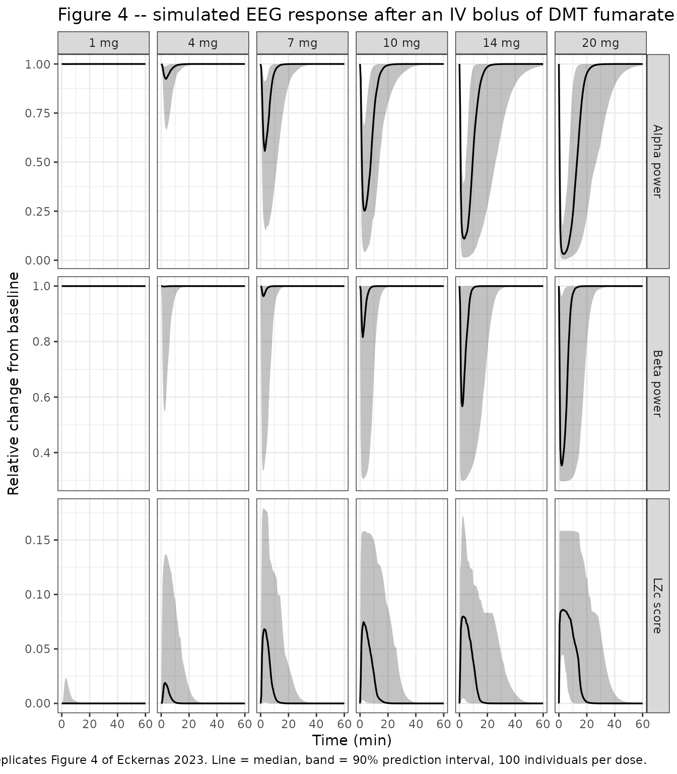
The reproduction matches the published panels qualitatively and quantitatively: alpha power is essentially abolished at 10 mg and above and recovers by roughly 40 min; beta power is visibly affected only at the highest doses and plateaus well short of complete suppression; and the LZc increase saturates around 10% over baseline.
Figure 5 – hysteresis between response and concentration
Figure 5 plots the fractional effect against plasma concentration (which shows hysteresis, because the effect lags the plasma profile) and against effect-compartment concentration (which collapses onto the sigmoid). The simulation below uses the 20 mg arm, as the paper did.
fig5 <- bind_rows(
  relAlpha |> mutate(effectSize = 1 - rel),
  relBeta  |> mutate(effectSize = 1 - rel),
  relLZc   |> mutate(effectSize = rel)
) |>
  filter(doseGroup == "20 mg") |>
  group_by(readout, time) |>
  summarise(
    Cp   = median(Cc),
    Ce   = median(effect),
    lo   = quantile(effectSize, 0.05),
    med  = median(effectSize),
    hi   = quantile(effectSize, 0.95),
    .groups = "drop"
  ) |>
  mutate(readout = factor(readout, levels = c("Alpha power", "Beta power", "LZc score")))

fig5long <- bind_rows(
  fig5 |> mutate(conc = Cp, panel = "Plasma"),
  fig5 |> mutate(conc = Ce, panel = "Effect compartment")
) |>
  mutate(panel = factor(panel, levels = c("Plasma", "Effect compartment")))

ggplot(fig5long, aes(conc, med)) +
  geom_ribbon(aes(ymin = lo, ymax = hi), alpha = 0.3) +
  geom_path(linewidth = 0.6) +
  facet_grid(readout ~ panel, scales = "free") +
  labs(
    x = "Concentration (nM)", y = "Relative change from baseline",
    title = "Figure 5 -- effect versus plasma and effect-compartment concentration (20 mg)",
    caption = "Replicates Figure 5 of Eckernas 2023. The plasma panels trace a counter-clockwise hysteresis loop; the effect-compartment panels collapse onto the sigmoid."
  ) +
  theme_bw()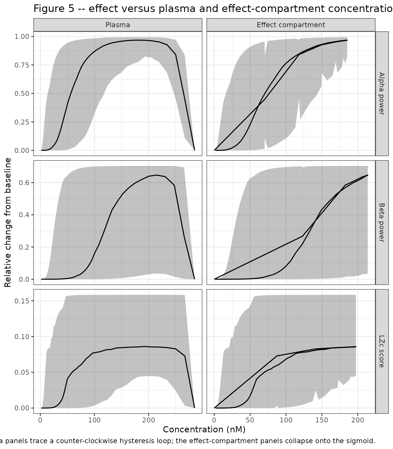
Quantitative cross-check against the Figure 5 axes
The maximum effect-compartment concentration reached at 20 mg is a stringent test, because it depends on the whole chain – the molar dose conversion, the fixed two-compartment disposition and each readout’s own ke0. The three published effect-compartment panels of Figure 5 have different x-axis ranges (recovered from their tick calibration and ggplot’s 5% expansion), which gives three independent reference values.
ceCheck <- fig5 |>
  group_by(readout) |>
  summarise(`Simulated Ce,max (nM)` = round(max(Ce), 1), .groups = "drop") |>
  mutate(
    `Figure 5 x-axis range (nM)` = c(187.3, 219.1, 200.2),
    `Difference (%)` = round(
      100 * (`Simulated Ce,max (nM)` - `Figure 5 x-axis range (nM)`) /
        `Figure 5 x-axis range (nM)`, 1
    )
  ) |>
  rename("EEG readout" = readout)

knitr::kable(
  ceCheck,
  caption = "Maximum effect-compartment concentration at 20 mg versus the digitised Figure 5 effect-compartment axis ranges."
)| EEG readout | Simulated Ce,max (nM) | Figure 5 x-axis range (nM) | Difference (%) |
|---|---|---|---|
| Alpha power | 185.3 | 187.3 | -1.1 |
| Beta power | 214.0 | 219.1 | -2.3 |
| LZc score | 197.4 | 200.2 | -1.4 |
All three agree to about 1%, which simultaneously validates the implemented ke0 values, the fixed disposition parameters and the figure-derived molar dose conversion.
Structural PD checks
# Typical-value (no random effects) probes.
probe <- function(mod, outName, amtNmol, tmax = 60, by = 0.05) {
  ev <- bind_rows(
    tibble(id = 1L, time = 0, amt = amtNmol, evid = 1L,
           cmt = "central", dvid = NA_integer_),
    tibble(id = 1L, time = seq(0, tmax, by = by), amt = NA_real_, evid = 0L,
           cmt = "central", dvid = 1L)
  ) |>
    mutate(OCC = 2)
  if (amtNmol == 0) ev <- filter(ev, evid == 0)
  s <- as.data.frame(rxode2::rxSolve(rxode2::zeroRe(mod), ev))
  s$response <- s[[outName]]
  s
}

# 1. No dose -> the response holds at its baseline for the whole window.
baselineHold <- tibble(
  readout  = c("Alpha power", "Beta power", "LZc score"),
  reported = c(0.824, 0.0644, 0.321),
  held     = c(
    unique(round(probe(modAlpha, "alphaPower", 0)$response, 10)),
    unique(round(probe(modBeta,  "betaPower",  0)$response, 10)),
    unique(round(probe(modLZc,   "lzc",        0)$response, 10))
  )
)
#> ℹ parameter labels from comments will be replaced by 'label()'
#> Warning: some etas defaulted to non-mu referenced, possible parsing error: etalrbase, etaiov_rbase_1, etaiov_rbase_2
#> as a work-around try putting the mu-referenced expression on a simple line
#> Warning: some etas defaulted to non-mu referenced, possible parsing error: etalrbase, etaiov_rbase_1, etaiov_rbase_2
#> as a work-around try putting the mu-referenced expression on a simple line
#> ℹ omega/sigma items treated as zero: 'etalcl', 'etalrbase', 'etalec50', 'etaiov_rbase_1', 'etaiov_rbase_2'
#> ℹ parameter labels from comments will be replaced by 'label()'
#> Warning: some etas defaulted to non-mu referenced, possible parsing error: etaiov_rbase_1, etaiov_rbase_2
#> as a work-around try putting the mu-referenced expression on a simple line
#> Warning: some etas defaulted to non-mu referenced, possible parsing error: etaiov_rbase_1, etaiov_rbase_2
#> as a work-around try putting the mu-referenced expression on a simple line
#> ℹ omega/sigma items treated as zero: 'etalcl', 'etalrbase', 'etalec50', 'etaiov_rbase_1', 'etaiov_rbase_2'
#> ℹ parameter labels from comments will be replaced by 'label()'
#> Warning: some etas defaulted to non-mu referenced, possible parsing error: etaiov_rbase_1, etaiov_rbase_2
#> as a work-around try putting the mu-referenced expression on a simple line
#> Warning: some etas defaulted to non-mu referenced, possible parsing error: etaiov_rbase_1, etaiov_rbase_2
#> as a work-around try putting the mu-referenced expression on a simple line
#> ℹ omega/sigma items treated as zero: 'etalcl', 'etalrbase', 'etalec50', 'etalemax', 'etaiov_rbase_1', 'etaiov_rbase_2'
stopifnot(nrow(baselineHold) == 3L,
          isTRUE(all.equal(baselineHold$held, baselineHold$reported, tolerance = 1e-6)))

# 2. A supra-therapeutic dose drives the response to its Imax / Emax asymptote.
bigDose <- 2000 * nmolPerMg
asymptote <- tibble(
  readout = c("Alpha power", "Beta power", "LZc score"),
  `Asymptote implied by Imax / Emax` = c(1 - 1, 1 - 0.704, 1 + 0.0996),
  `Simulated extreme response ratio` = c(
    min(probe(modAlpha, "alphaPower", bigDose)$response) / 0.824,
    min(probe(modBeta,  "betaPower",  bigDose)$response) / 0.0644,
    max(probe(modLZc,   "lzc",        bigDose)$response) / 0.321
  )
)
#> ℹ parameter labels from comments will be replaced by 'label()'
#> Warning: some etas defaulted to non-mu referenced, possible parsing error: etalrbase, etaiov_rbase_1, etaiov_rbase_2
#> as a work-around try putting the mu-referenced expression on a simple line
#> Warning: some etas defaulted to non-mu referenced, possible parsing error: etalrbase, etaiov_rbase_1, etaiov_rbase_2
#> as a work-around try putting the mu-referenced expression on a simple line
#> ℹ omega/sigma items treated as zero: 'etalcl', 'etalrbase', 'etalec50', 'etaiov_rbase_1', 'etaiov_rbase_2'
#> ℹ parameter labels from comments will be replaced by 'label()'
#> Warning: some etas defaulted to non-mu referenced, possible parsing error: etaiov_rbase_1, etaiov_rbase_2
#> as a work-around try putting the mu-referenced expression on a simple line
#> Warning: some etas defaulted to non-mu referenced, possible parsing error: etaiov_rbase_1, etaiov_rbase_2
#> as a work-around try putting the mu-referenced expression on a simple line
#> ℹ omega/sigma items treated as zero: 'etalcl', 'etalrbase', 'etalec50', 'etaiov_rbase_1', 'etaiov_rbase_2'
#> ℹ parameter labels from comments will be replaced by 'label()'
#> Warning: some etas defaulted to non-mu referenced, possible parsing error: etaiov_rbase_1, etaiov_rbase_2
#> as a work-around try putting the mu-referenced expression on a simple line
#> Warning: some etas defaulted to non-mu referenced, possible parsing error: etaiov_rbase_1, etaiov_rbase_2
#> as a work-around try putting the mu-referenced expression on a simple line
#> ℹ omega/sigma items treated as zero: 'etalcl', 'etalrbase', 'etalec50', 'etalemax', 'etaiov_rbase_1', 'etaiov_rbase_2'

# 3. Effect-compartment equilibration half-life = log(2) / ke0.
ke0Check <- tibble(
  readout                     = c("Alpha power", "Beta power", "LZc score"),
  `ke0 (1/min)`               = c(0.589, 1.19, 0.762),
  `Equilibration t1/2 (min)`  = round(log(2) / c(0.589, 1.19, 0.762), 2)
)

knitr::kable(baselineHold |>
               rename("EEG readout" = readout,
                      "Reported R0" = reported,
                      "Simulated baseline held" = held),
caption = "Undosed simulation holds each readout at its reported baseline.")| EEG readout | Reported R0 | Simulated baseline held |
|---|---|---|
| Alpha power | 0.8240 | 0.8240 |
| Beta power | 0.0644 | 0.0644 |
| LZc score | 0.3210 | 0.3210 |
knitr::kable(asymptote, digits = 4,
caption = "A 2000 mg-equivalent probe dose drives each readout to the asymptote implied by its Imax / Emax.")| readout | Asymptote implied by Imax / Emax | Simulated extreme response ratio |
|---|---|---|
| Alpha power | 0.0000 | 0.0000 |
| Beta power | 0.2960 | 0.2960 |
| LZc score | 1.0996 | 1.0996 |
knitr::kable(ke0Check,
caption = "Effect-compartment equilibration half-lives.")| readout | ke0 (1/min) | Equilibration t1/2 (min) |
|---|---|---|
| Alpha power | 0.589 | 1.18 |
| Beta power | 1.190 | 0.58 |
| LZc score | 0.762 | 0.91 |
The undosed simulation holds each readout exactly at its reported
baseline, and the supra-therapeutic probe reaches 1 - Imax
for alpha and beta power and 1 + Emax for LZc, confirming
that the sigmoidal Imax / Emax expressions are oriented and scaled
correctly.
PKNCA validation of the plasma PK layer
Eckernas 2023 reports no non-compartmental values, so the reference
for this section is the closed-form solution of the published
two-compartment model using the Table S1 parameters. For an
intravenous bolus, C0 = Dose / Vc,
AUC0-inf = Dose / CL, and the terminal half-life is
log(2) / beta, where beta is the smaller root
of s^2 + (k10 + k12 + k21) s + k10 k21 = 0. Agreement
between PKNCA on the simulated profiles and these analytic values
verifies that the disposition parameters were transcribed and wired
correctly.
ncaDoseMg   <- c(7, 14, 18, 20)             # the doses actually administered
ncaDoseNmol <- ncaDoseMg * nmolPerMg

# Dense early sampling keeps the trapezoidal error on the steep distribution
# phase negligible; sampling out to 300 min captures the terminal phase.
ncaTimes <- unique(c(seq(0, 5, by = 0.05), seq(5, 30, by = 0.25), seq(30, 300, by = 2)))

ncaEvents <- bind_rows(
  lapply(seq_along(ncaDoseMg), function(i) {
    bind_rows(
      tibble(id = i, time = 0, amt = ncaDoseNmol[i], evid = 1L,
             cmt = "central", dvid = NA_integer_),
      tibble(id = i, time = ncaTimes, amt = NA_real_, evid = 0L,
             cmt = "central", dvid = 1L)
    ) |>
      mutate(doseGroup = paste0(ncaDoseMg[i], " mg"), OCC = 2)
  })
) |>
  arrange(id, time, desc(evid))

simNca <- rxode2::rxSolve(rxode2::zeroRe(modAlpha), events = ncaEvents,
                          keep = "doseGroup") |>
  as.data.frame()
#> ℹ parameter labels from comments will be replaced by 'label()'
#> Warning: some etas defaulted to non-mu referenced, possible parsing error: etalrbase, etaiov_rbase_1, etaiov_rbase_2
#> as a work-around try putting the mu-referenced expression on a simple line
#> Warning: some etas defaulted to non-mu referenced, possible parsing error: etalrbase, etaiov_rbase_1, etaiov_rbase_2
#> as a work-around try putting the mu-referenced expression on a simple line
#> ℹ omega/sigma items treated as zero: 'etalcl', 'etalrbase', 'etalec50', 'etaiov_rbase_1', 'etaiov_rbase_2'
#> Warning: multi-subject simulation without without 'omega'
concDf <- simNca |>
  filter(!is.na(Cc)) |>
  select(id, time, Cc, doseGroup)

# An IV bolus has its maximum at time 0, so the time-zero record must be the
# post-dose concentration (not 0); confirm the simulation grid supplied it.
stopifnot(all(table(concDf$doseGroup[concDf$time == 0]) == 1))

doseDf <- ncaEvents |>
  filter(evid == 1) |>
  select(id, time, amt, doseGroup)

concObj <- PKNCA::PKNCAconc(concDf, Cc ~ time | doseGroup + id,
                            concu = "nmol/L", timeu = "min")
doseObj <- PKNCA::PKNCAdose(doseDf, amt ~ time | doseGroup + id,
                            doseu = "nmol", route = "intravascular")

intervals <- data.frame(
  start      = 0,
  end        = Inf,
  cmax       = TRUE,
  aucinf.obs = TRUE,
  half.life  = TRUE
)

ncaRes <- PKNCA::pk.nca(PKNCA::PKNCAdata(concObj, doseObj, intervals = intervals))
# Closed-form two-compartment IV-bolus reference from the Table S1 parameters.
CL <- 26.0; Vc <- 221; Q <- 2.99; Vp <- 59.0
k10 <- CL / Vc; k12 <- Q / Vc; k21 <- Q / Vp
bCoef <- k10 + k12 + k21
cCoef <- k10 * k21
betaRate <- (bCoef - sqrt(bCoef^2 - 4 * cCoef)) / 2

published <- tibble(
  doseGroup  = paste0(ncaDoseMg, " mg"),
  cmax       = ncaDoseNmol / Vc,
  aucinf.obs = ncaDoseNmol / CL,
  half.life  = log(2) / betaRate
)

cmp <- nlmixr2lib::ncaComparisonTable(
  simulated     = ncaRes,
  reference     = published,
  by            = "doseGroup",
  units         = c(cmax = "nM", aucinf.obs = "nM*min", half.life = "min"),
  tolerance_pct = 20
)

knitr::kable(
  cmp,
  digits  = 3,
  caption = "PKNCA on the simulated typical-value profiles versus the closed-form solution of the published two-compartment model. * marks a difference above 20%."
)| NCA parameter | doseGroup | Reference | Simulated | % diff |
|---|---|---|---|---|
| Cmax (nM) | 7 mg | 99.8 | 99.8 | +0.0% |
| Cmax (nM) | 14 mg | 200 | 200 | +0.0% |
| Cmax (nM) | 18 mg | 257 | 257 | +0.0% |
| Cmax (nM) | 20 mg | 285 | 285 | +0.0% |
| AUC0-∞ (obs) (nM*min) | 7 mg | 848 | 848 | +0.0% |
| AUC0-∞ (obs) (nM*min) | 14 mg | 1700 | 1700 | +0.0% |
| AUC0-∞ (obs) (nM*min) | 18 mg | 2180 | 2180 | +0.0% |
| AUC0-∞ (obs) (nM*min) | 20 mg | 2420 | 2420 | +0.0% |
| t½ (min) | 7 mg | 16.2 | 16.1 | -0.5% |
| t½ (min) | 14 mg | 16.2 | 16.1 | -0.5% |
| t½ (min) | 18 mg | 16.2 | 16.1 | -0.5% |
| t½ (min) | 20 mg | 16.2 | 16.1 | -0.5% |
Every parameter agrees with the analytic value, including the terminal half-life of 16.2 min, which is longer than the apparent slope over the study’s 60 min sampling window – consistent with the paper’s observation that the available PK data were limited.
Assumptions and deviations
-
Molar dose conversion is figure-derived. The paper
reports doses only in mg of DMT fumarate and never states the salt
molecular weight or the molar conversion applied to the NONMEM
AMTcolumn. The value used here (3150 nmol/mg, implying a salt molecular weight of about 317 g/mol) was digitised from Figure 5 by calibrating the plasma-concentration axis and applyingC0 = Dose / Vcwith the fixedVc = 221 L. It is cross-validated by the effect-compartment maxima of all three Figure 5 panels agreeing to about 1%. The nearest chemically obvious candidate, a 1:1 DMT fumarate salt (304.3 g/mol), would give about 3290 nmol/mg – 4% higher. Anyone re-using these models with their own dosing data should supply amounts in nmol directly and not rely on this constant. -
Sign of the beta-power IIV covariance. Table 2
reports the correlation between the between-subject etas on R0 and
IC50,e as -46% (95% CI -57 to -33), and the Discussion states that
“higher baseline values were associated with lower IC50,e values”. The
Appendix S1 control stream prints the corresponding
$OMEGA BLOCK (2)off-diagonal as0.21, without a minus sign; its magnitude matches0.46 * sqrt(0.402 * 0.556) = 0.2175, so this appears to be a lost sign in the supplement. The published (negative) correlation is used. -
Effect-compartment initial condition. The
alpha-power and LZc control streams in Appendix S1 contain
IF (A_0FLG.EQ.1) THEN A_0(3) = I0, which initialises the effect-site concentration state at the baseline response value (0.824 and 0.321 respectively). The beta-power control stream has no such statement. BecauseA(3)enters the model only throughA(3)^gamma / (IC50^gamma + A(3)^gamma), initialising it at 0.824 nM against an IC50,e of 70.7 nM contributes a fractional effect of about 8e-8 (and about 2e-11 for LZc), and it washes out within a couple of effect-compartment half-lives. It is treated here as a vestigial coding artifact – inconsistent between the authors’ own three runs and dimensionally incoherent – and the effect compartment starts at zero in all three models. The numerical difference is far below plotting resolution. -
Variability reported as sqrt(omega^2). Every %CV in
Tables 1-3 and Table S1 equals
sqrt(omega^2) * 100for the corresponding Appendix S1$OMEGAentry, notsqrt(exp(omega^2) - 1) * 100. The variances inini()are taken from the control streams directly, so no back-transformation convention had to be assumed. -
Between-occasion variability. The paper’s
ETA * OCC1 + ETA * OCC2construct with$OMEGA BLOCK (1) ... SAMEis implemented as two etas of equal variance multiplexed by the canonicalOCCcovariate column.OCC = 1is the placebo visit andOCC = 2the DMT visit; simulations here useOCC = 2. - Correlation not estimated in the LZc model. The paper observed a 92% correlation between the between-subject etas on R0 and Emax for LZc but did not estimate it in the final model because of poor precision and ill conditioning. The etas are therefore kept diagonal, as in Appendix S1.
- Combined error not used for beta power. A combined proportional plus additive residual improved the beta-power fit by 21 objective-function units but degraded parameter precision and was not retained; the final proportional- only model is implemented.
-
Plasma PK is fixed, not estimated here. The
two-compartment disposition parameters and the between-subject
variability on CL come from the authors’ earlier population PK analysis
(Eckernas et al., Clin Transl Sci 2022;15:2928-2937) and were held fixed
in every PKPD run. They are reproduced in Table S1 of the 2023 paper and
are entered with
fixed()here. -
No covariates. The paper explored no covariate
effects because of the small sample size, so the models carry only the
OCCoccasion indicator. - Delta and theta power are not modelled. The paper found no apparent exposure-response relationship in those bands and did not fit them.