Amoxicillin in maternal, umbilical cord and neonatal serum (Muller 2009)
Source:vignettes/articles/Muller_2009_amoxicillin.Rmd
Muller_2009_amoxicillin.RmdModel and source
- Citation: Muller AE, Oostvogel PM, DeJongh J, Mouton JW, Steegers EAP, Dorr PJ, Danhof M, Voskuyl RA. Pharmacokinetics of amoxicillin in maternal, umbilical cord, and neonatal sera. Antimicrob Agents Chemother. 2009;53(4):1574-1580. doi:10.1128/AAC.00119-08.
- Description: Five-compartment population PK model for intravenous amoxicillin in labouring women, the venous umbilical cord and the neonate, fitted simultaneously to maternal, arterial and venous umbilical cord and neonatal serum concentrations. Three maternal compartments (central V1 plus two peripheral compartments constrained to a common volume V2 = V3) exchange with a venous umbilical cord compartment V4 via the transplacental rate constants k14 / k41; a neonatal compartment V5 hangs off the cord compartment via k45 / k54 and eliminates drug from the system via k50. Central volume increases 4.2% per week of gestational age (Muller 2009).
- Article: https://doi.org/10.1128/AAC.00119-08
This is the first published model in which maternal, umbilical cord
and neonatal amoxicillin concentrations were fitted
simultaneously. It is the successor to
Muller_2008_amoxicillin, the three-compartment maternal
model developed in women with preterm premature rupture of membranes;
the 2009 analysis reuses 416 of those maternal samples and adds the cord
and neonatal data that the earlier analysis did not use.
Population
Between 7 February 2005 and 28 February 2007, 44 pregnant women at Medical Centre Haaglanden (The Hague, the Netherlands) received intravenous amoxicillin (or co-amoxiclav) shortly before or during labour, for prevention of neonatal group B streptococcal (GBS) disease or for suspected intra-amniotic infection. Maternal age was 30.0 +/- 6.85 years, body weight 79.4 +/- 13.9 kg, body mass index 29.4 +/- 5.3 kg/m^2, and mean amenorrhoea 36 6/7 weeks (SD 2.7); deliveries occurred at gestational ages of 30.0 to 42.4 weeks and neonatal birth weights of 1340 to 4470 g (Muller 2009 Table 1, Results paragraph 1).
The amoxicillin regimen was 2 g (50 mg/mL) over a 30-min IV infusion followed 4 h later by 1 g over 15 min; the co-amoxiclav regimen was 1 g amoxicillin with 200 mg clavulanic acid over 15 min every 8 h. The two groups were pooled because clavulanic acid does not alter intravenous amoxicillin PK.
The analysis dataset comprised 904 maternal serum samples (3-41 per patient), 53 umbilical cord samples (25 arterial and 28 venous; both from 23 women), and 14 neonatal heel-puncture samples from 13 neonates taken 14.2-199.8 min after birth. The interval between the last maternal dose and birth ranged from 24.4 to 316.8 min. The assay LLOQ was 0.2 mg/L with a between-run CV below 4%.
Programmatic access:
muller_pop <- rxode2::rxode(readModelDb("Muller_2009_amoxicillin"))$population
#> ℹ parameter labels from comments will be replaced by 'label()'
muller_pop[c("species", "n_subjects", "n_observations", "age_range",
             "weight_range", "ga_range", "dose_range")]
#> $species
#> [1] "human"
#>
#> $n_subjects
#> [1] 44
#>
#> $n_observations
#> [1] 971
#>
#> $age_range
#> [1] "mean 30.0 +/- 6.85 years (maternal age, n = 44)"
#>
#> $weight_range
#> [1] "mean 79.4 +/- 13.9 kg (n = 43)"
#>
#> $ga_range
#> [1] "30.0-42.4 weeks at delivery; cohort mean amenorrhoea 36 6/7 weeks (SD 2.7)"
#>
#> $dose_range
#> [1] "Amoxicillin 2 g IV over 30 min followed after 4 h by 1 g IV over 15 min; or co-amoxiclav (1 g amoxicillin with 200 mg clavulanic acid) IV over 15 min every 8 h. All infusions at 50 mg/mL."
Model structure
Muller 2009 Figure 2 draws a five-compartment mass-transfer system:
- the maternal central compartment
central(V1), from which amoxicillin is cleared with CL and into which the infusion is delivered; - two maternal peripheral compartments
peripheral1(V2) andperipheral2(V3), exchanging withcentralthrough Q1 and Q2. Their volumes were “comparable (difference in the final model with separate estimates for V2 and V3, < 0.5 liter)” with coefficients of variation above 51%, so V3 was constrained equal to V2; - the venous umbilical cord compartment
cord_venous(V4), exchanging with the maternal central compartment through the transplacental rate constantsk14andk41; - the neonatal compartment
neonate(V5), hanging offcord_venousthroughk45andk54and eliminating drug from the system throughk50.
Because “only venous cord blood enters the umbilical cord after passage through the placenta, the antibiotic exchange between the compartments might not be equal”, the authors parameterised the fetal side with first-order rate constants rather than intercompartmental clearances (Methods, “PK analysis”). The subscripts are the NONMEM ADVAN5 slot indices of Figure 2 and are kept verbatim as the model’s parameter names.
Two structural simplifications carried over from the paper are worth noting. Arterial and venous cord concentrations were not separated, because their ratio was not significantly different from 1 (Figure 1) and “the differences … were too small for analysis of these concentrations by the use of two separate compartments”. The arterial cord samples were then pooled with the neonatal samples into compartment 5, since “arterial cord blood originates directly from the fetal circulation”.
Source trace
Per-parameter origin is also recorded as in-file comments in
inst/modeldb/specificDrugs/Muller_2009_amoxicillin.R.
| Equation / parameter | Value (typical) | Source location |
|---|---|---|
lcl |
log(19.7) L/h |
Table 2 row CL (SE 0.99, CI 17.8-21.6); Abstract |
lvc |
log(6.40) L |
Table 2 row V1 (SE 0.61, CI 5.2-7.6); Abstract |
lvp |
log(5.88) L |
Table 2 row V2 (SE 0.83, CI 4.2-7.5); Abstract |
lvp2 |
log(5.88) L |
Table 2 row V3, constrained V3 = V2 (Results paragraph 3) |
lq |
log(56.6) L/h |
Table 2 row Q1 (SE 9.5, CI 38.0-75.2) |
lq2 |
log(10.7) L/h |
Table 2 row Q2 (SE 2.2, CI 6.3-15.1) |
lk14 |
log(0.76) 1/h |
Table 2 row k14 (SE 0.28, CI 0.21-1.3) |
lk41 |
log(1.4) 1/h |
Table 2 row k41 (SE 0.31, CI 0.83-2.1) |
lk45 |
log(5.1) 1/h |
Table 2 row k45 (SE 2, CI 1.1-9.1) |
lk54 |
log(1.4) 1/h |
Table 2 row k54 (SE 0.31, CI 0.83-2.1) |
lk50 |
log(0.16) 1/h |
Table 2 row k50 (SE 0.033, CI 0.098-0.23) |
lv4 |
fixed(log(3.4)) L |
Results paragraph 4 (“3.4 liters for the venous umbilical cord”) |
lv5 |
fixed(log(11.9)) L |
Results paragraph 4 (“11.9 liters for the neonate”) |
e_ga_vc |
0.042 per week |
Results paragraph 4 (“An increase in V1 of 4.2% per week”) |
etalcl variance |
0.076 |
Table 2 row Interindividual variability in CL (SE
0.026, CI 0.026-0.13) |
etalvc variance |
0.038 |
Table 2 row Interindividual variability in V1 (SE
0.013, CI 0.014-0.063) |
propSd, propSd_Ccord,
propSd_Cneonate
|
sqrt(0.03) (= 0.173, 17.3%) |
Table 2 row Residual variability (SE 0.004, CI
0.022-0.037); one proportional model shared by all matrices (Methods “PK
analysis”) |
| Five-compartment ODE system | see model()
|
Figure 2 and Results paragraph 3 |
| V1 covariate adjustment | V1 = theta2 * [1 + theta12 * (GA - 36.8)] * exp(eta2) |
Results paragraph 4, printed equation |
Every 95% confidence interval in Table 2 is a Wald interval
Mean +/- 1.96 * SE, which is used below as an independent
transcription check on the rotated (landscape) table.
The check has to respect the table’s own precision. Every entry is
printed to two significant figures, so each printed number stands for an
interval (k45’s SE of 2 means anything in
[1.5, 2.5]), and a naive Mean - 1.96 * SE computed from the
rounded values need not land on the rounded bound. The
comparison below is therefore interval-valued: the range of
Mean +/- 1.96 * SE attainable over the rounding intervals
of the mean and the SE must overlap the rounding interval of the printed
bound. This is strictly tighter than a blanket tolerance – a single
mistyped digit in any of the four columns breaks the overlap – and all
14 rows satisfy it.
# Values are carried as the strings Table 2 actually prints, so the
# rounding interval of each can be recovered from its precision.
tab2 <- tibble::tribble(
  ~parameter, ~mean,   ~se,     ~lo,     ~hi,
  "CL",       "19.7",  "0.99",  "17.8",  "21.6",
  "V1",       "6.4",   "0.61",  "5.2",   "7.6",
  "V2",       "5.88",  "0.83",  "4.2",   "7.5",
  "V3",       "5.88",  "0.83",  "4.2",   "7.5",
  "Q1",       "56.6",  "9.5",   "38.0",  "75.2",
  "Q2",       "10.7",  "2.2",   "6.3",   "15.1",
  "k14",      "0.76",  "0.28",  "0.21",  "1.3",
  "k41",      "1.4",   "0.31",  "0.83",  "2.1",
  "k45",      "5.1",   "2",     "1.1",   "9.1",
  "k54",      "1.4",   "0.31",  "0.83",  "2.1",
  "k50",      "0.16",  "0.033", "0.098", "0.23",
  "IIV CL",   "0.076", "0.026", "0.026", "0.13",
  "IIV V1",   "0.038", "0.013", "0.014", "0.063",
  "Residual", "0.03",  "0.004", "0.022", "0.037"
)

# Half-width of the rounding interval implied by a printed number's own
# precision: "38.0" -> 0.05, "2" -> 0.5, "0.033" -> 0.0005.
round_halfwidth <- function(x) {
  dec <- ifelse(grepl(".", x, fixed = TRUE),
                nchar(sub("^[^.]*\\.", "", x)), 0L)
  0.5 * 10^(-dec)
}

ci_chk <- tab2 |>
  mutate(across(c(mean, se, lo, hi), as.numeric,        .names = "{.col}_v"),
         across(c(mean, se, lo, hi), round_halfwidth,   .names = "{.col}_h")) |>
  mutate(
    # Range of Mean -/+ 1.96*SE over the rounding intervals of both.
    lo_min = mean_v - mean_h - 1.96 * (se_v + se_h),
    lo_max = mean_v + mean_h - 1.96 * (se_v - se_h),
    hi_min = mean_v - mean_h + 1.96 * (se_v - se_h),
    hi_max = mean_v + mean_h + 1.96 * (se_v + se_h),
    # ... must overlap the rounding interval of the printed bound.
    lo_ok  = lo_min <= lo_v + lo_h & lo_max >= lo_v - lo_h,
    hi_ok  = hi_min <= hi_v + hi_h & hi_max >= hi_v - hi_h
  )

# Deterministic check on the transcribed table, not on any simulation.
stopifnot(all(ci_chk$lo_ok), all(ci_chk$hi_ok))

ci_chk |>
  mutate(across(c(lo_min, lo_max, hi_min, hi_max), \(x) signif(x, 3))) |>
  select(parameter, mean, se, lo, lo_min, lo_max, lo_ok,
         hi, hi_min, hi_max, hi_ok) |>
  rename("Parameter" = parameter, "Mean" = mean, "SE" = se,
         "CI lower (printed)" = lo,
         "Attainable lower, min" = lo_min,
         "Attainable lower, max" = lo_max,
         "Lower OK" = lo_ok,
         "CI upper (printed)" = hi,
         "Attainable upper, min" = hi_min,
         "Attainable upper, max" = hi_max,
         "Upper OK" = hi_ok) |>
knitr::kable()| Parameter | Mean | SE | CI lower (printed) | Attainable lower, min | Attainable lower, max | Lower OK | CI upper (printed) | Attainable upper, min | Attainable upper, max | Upper OK |
|---|---|---|---|---|---|---|---|---|---|---|
| CL | 19.7 | 0.99 | 17.8 | 17.7000 | 17.8000 | TRUE | 21.6 | 21.6000 | 21.7000 | TRUE |
| V1 | 6.4 | 0.61 | 5.2 | 5.1400 | 5.2600 | TRUE | 7.6 | 7.5400 | 7.6600 | TRUE |
| V2 | 5.88 | 0.83 | 4.2 | 4.2400 | 4.2700 | TRUE | 7.5 | 7.4900 | 7.5200 | TRUE |
| V3 | 5.88 | 0.83 | 4.2 | 4.2400 | 4.2700 | TRUE | 7.5 | 7.4900 | 7.5200 | TRUE |
| Q1 | 56.6 | 9.5 | 38.0 | 37.8000 | 38.1000 | TRUE | 75.2 | 75.1000 | 75.4000 | TRUE |
| Q2 | 10.7 | 2.2 | 6.3 | 6.2400 | 6.5400 | TRUE | 15.1 | 14.9000 | 15.2000 | TRUE |
| k14 | 0.76 | 0.28 | 0.21 | 0.1960 | 0.2260 | TRUE | 1.3 | 1.2900 | 1.3200 | TRUE |
| k41 | 1.4 | 0.31 | 0.83 | 0.7330 | 0.8520 | TRUE | 2.1 | 1.9500 | 2.0700 | TRUE |
| k45 | 5.1 | 2 | 1.1 | 0.1500 | 2.2100 | TRUE | 9.1 | 7.9900 | 10.0000 | TRUE |
| k54 | 1.4 | 0.31 | 0.83 | 0.7330 | 0.8520 | TRUE | 2.1 | 1.9500 | 2.0700 | TRUE |
| k50 | 0.16 | 0.033 | 0.098 | 0.0893 | 0.1010 | TRUE | 0.23 | 0.2190 | 0.2310 | TRUE |
| IIV CL | 0.076 | 0.026 | 0.026 | 0.0236 | 0.0265 | TRUE | 0.13 | 0.1250 | 0.1280 | TRUE |
| IIV V1 | 0.038 | 0.013 | 0.014 | 0.0110 | 0.0140 | TRUE | 0.063 | 0.0620 | 0.0650 | TRUE |
| Residual | 0.03 | 0.004 | 0.022 | 0.0162 | 0.0281 | TRUE | 0.037 | 0.0319 | 0.0438 | TRUE |
The two derived fetal-side volumes
ADVAN5 estimates only rate constants for the fetal-side slots, so V4
and V5 are not in Table 2. Results paragraph 4 states that they “were
calculated and were found to be 3.4 liters for the venous umbilical cord
and 11.9 liters for the neonate”, without printing the formula. Both are
recovered by the flow-balance identity implied by Figure 2 – passive
exchange across a boundary carries the same clearance in each direction,
so k14 * V1 = k41 * V4 and
k45 * V4 = k54 * V5.
This is also the check that fixes the direction of every
rate constant: transposing k14 and k41 would
give V4 = 11.8 L, three and a half times the published value.
k <- list(V1 = 6.4, k14 = 0.76, k41 = 1.4, k45 = 5.1, k54 = 1.4)
v4_calc <- k$k14 * k$V1 / k$k41
v5_calc <- k$k45 * 3.4 / k$k54

stopifnot(
  # Deterministic arithmetic on published point estimates -- no
  # simulation, no cohort, so the bounds are tight. The residual gap is
  # entirely the two-significant-figure rounding of the k values.
  abs(v4_calc - 3.4)  / 3.4  < 0.03,
  abs(v5_calc - 11.9) / 11.9 < 0.05
)
tibble::tibble(
  Volume = c("V4 (venous umbilical cord)", "V5 (neonate)"),
  `Flow-balance identity` = c("k14 * V1 / k41", "k45 * V4 / k54"),
  `Recomputed (L)` = signif(c(v4_calc, v5_calc), 4),
  `Published (L)` = c(3.4, 11.9)
) |>
knitr::kable()| Volume | Flow-balance identity | Recomputed (L) | Published (L) |
|---|---|---|---|
| V4 (venous umbilical cord) | k14 * V1 / k41 | 3.474 | 3.4 |
| V5 (neonate) | k45 * V4 / k54 | 12.390 | 11.9 |
Transposing k14 and k41 is ruled out
explicitly:
Typical-value simulation of the published scenario
Muller 2009 Figure 4 simulates a single 2 g maternal infusion over 30 min and follows all three matrices. The chunk below reproduces that scenario from the library model with the between-subject random effects zeroed.
The event table doses cmt = "central" (an ODE state) and
places observation records on the Cc endpoint. This model
declares three endpoints (Cc, Ccord,
Cneonate), so rxode2 requires observation rows to name an
endpoint rather than an ODE state; one endpoint suffices, because every
algebraic observable is returned as its own column at every observation
row.
mod <- readModelDb("Muller_2009_amoxicillin")
mod_typ <- rxode2::zeroRe(mod)
#> ℹ parameter labels from comments will be replaced by 'label()'

obs_times <- sort(unique(c(seq(0, 4, by = 0.005), seq(4, 72, by = 0.02))))
ev_typ <- rxode2::et(amt = 2000, dur = 0.5, cmt = "central")
ev_typ <- rxode2::et(ev_typ, obs_times, cmt = "Cc")
ev_typ <- as.data.frame(ev_typ)
ev_typ$GA <- 36.8  # the median GA on which the covariate model is centred

sim_typ <- rxode2::rxSolve(mod_typ, ev_typ, returnType = "data.frame") |>
  dplyr::filter(!is.na(Cc))
#> ℹ omega/sigma items treated as zero: 'etalcl', 'etalvc'

peak_of <- function(x, t) c(cmax = max(x), tmax = t[which.max(x)])
peaks <- rbind(
  Maternal = peak_of(sim_typ$Cc, sim_typ$time),
  Cord     = peak_of(sim_typ$Ccord, sim_typ$time),
  Neonate  = peak_of(sim_typ$Cneonate, sim_typ$time)
)
signif(peaks, 4)
#>           cmax  tmax
#> Maternal 92.25 0.500
#> Cord     19.53 0.585
#> Neonate  13.21 1.640
Replicates Figure 4 of Muller 2009
sim_typ |>
  dplyr::select(time, Mother = Cc, Cord = Ccord, Neonate = Cneonate) |>
  tidyr::pivot_longer(-time, names_to = "Matrix", values_to = "conc") |>
  dplyr::filter(time <= 10, conc >= 0.01) |>
  ggplot(aes(time, conc, linetype = Matrix)) +
  geom_line(linewidth = 0.6) +
  geom_hline(yintercept = 0.25, colour = "firebrick", linetype = "dotted") +
  annotate("text", x = 9.6, y = 0.30, hjust = 1, size = 3, colour = "firebrick",
           label = "EUCAST GBS breakpoint 0.25 mg/L") +
  scale_y_log10(limits = c(0.01, 200)) +
  labs(x = "Time (h)", y = "Amoxicillin concentration (mg/L)",
       title = "Replicates Figure 4 of Muller 2009",
       caption = paste("Typical-value profiles after a single 2 g maternal",
                       "infusion over 30 min. See 'Assumptions and",
                       "deviations' for the discrepancy against the",
                       "published Figure 4."))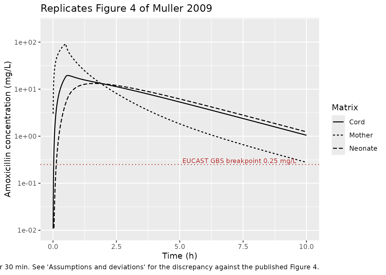
Qualitative behaviour reported in the text
Two qualitative statements in Results paragraph 6 and Discussion paragraph 1 are reproduced: the cord peak lags the maternal peak, and the neonatal concentration overtakes the cord concentration and stays above it thereafter.
cross <- with(sim_typ, {
  d <- Cneonate - Ccord
  time[which(d[-1] > 0 & d[-length(d)] <= 0)[1] + 1]
})

stopifnot(
  # Deterministic (typical-value) profile, so these are exact orderings,
  # not cohort quantiles.
  peaks["Maternal", "tmax"] == 0.5,                       # peak at end of infusion
  peaks["Cord", "tmax"] > peaks["Maternal", "tmax"],      # cord peak is delayed
  peaks["Cord", "cmax"] < peaks["Maternal", "cmax"],      # and lower
  peaks["Neonate", "tmax"] > peaks["Cord", "tmax"],       # neonatal peak later still
  cross > 1, cross < 3,                                   # neonate overtakes cord
  all(sim_typ$Cneonate[sim_typ$time > cross] >
        sim_typ$Ccord[sim_typ$time > cross])              # and stays above
)
sprintf("Cneonate exceeds Ccord from t = %.2f h onward", cross)
#> [1] "Cneonate exceeds Ccord from t = 1.99 h onward"
Comparison against the published simulated peaks
The values below are reported in Results paragraphs 5-7 as outputs of a separate Berkeley Madonna simulation (Methods, “Simulations”), not as parameter estimates. They are reported here for transparency; see “Assumptions and deviations” for why they are not asserted.
tibble::tibble(
  Quantity = c("Maternal Cmax (mg/L)", "Maternal tmax (h)",
               "Cord Cmax (mg/L)", "Cord peak delay after maternal peak (min)",
               "Cord/maternal peak ratio (%)", "Neonatal Cmax (mg/L)"),
  `Published (Berkeley Madonna)` = c(88.7, 0.5, 16.0, 3.3, 18, 8.0),
  `This model (rxode2)` = signif(c(
    peaks["Maternal", "cmax"], peaks["Maternal", "tmax"],
    peaks["Cord", "cmax"],
    60 * (peaks["Cord", "tmax"] - peaks["Maternal", "tmax"]),
    100 * peaks["Cord", "cmax"] / peaks["Maternal", "cmax"],
    peaks["Neonate", "cmax"]
  ), 4)
) |>
  mutate(`% diff` = signif(
    100 * (`This model (rxode2)` - `Published (Berkeley Madonna)`) /
      `Published (Berkeley Madonna)`, 3)) |>
knitr::kable()| Quantity | Published (Berkeley Madonna) | This model (rxode2) | % diff |
|---|---|---|---|
| Maternal Cmax (mg/L) | 88.7 | 92.25 | 4.0 |
| Maternal tmax (h) | 0.5 | 0.50 | 0.0 |
| Cord Cmax (mg/L) | 16.0 | 19.53 | 22.1 |
| Cord peak delay after maternal peak (min) | 3.3 | 5.10 | 54.5 |
| Cord/maternal peak ratio (%) | 18.0 | 21.17 | 17.6 |
| Neonatal Cmax (mg/L) | 8.0 | 13.21 | 65.1 |
Mass balance
Every milligram of the maternal dose leaves the system either through
the maternal clearance CL or through the neonatal elimination rate
constant k50. That gives an exact identity linking the two
AUCs to the dose,
Dose = CL * AUC(0-Inf, maternal) + k50 * V5 * AUC(0-Inf, neonatal),
which is an unusually sharp check because it exercises the ODE right-hand sides, both scaling volumes and the solver simultaneously. It is evaluated below from PKNCA output rather than from an inline trapezoid.
PKNCA validation
The source paper reports no NCA parameters, so PKNCA is used here for
structural verification rather than for a published-vs-simulated
comparison. The filter is !is.na(Cc) only, so the time-zero
record that anchors AUC(0-Inf) is retained.
nca_conc <- dplyr::bind_rows(
  tibble::tibble(id = 1L, matrix = "Maternal serum",
                 time = sim_typ$time, conc = sim_typ$Cc),
  tibble::tibble(id = 1L, matrix = "Venous umbilical cord serum",
                 time = sim_typ$time, conc = sim_typ$Ccord),
  tibble::tibble(id = 1L, matrix = "Neonatal serum",
                 time = sim_typ$time, conc = sim_typ$Cneonate)
) |>
  dplyr::filter(!is.na(conc))

nca_dose <- tibble::tibble(id = 1L, matrix = unique(nca_conc$matrix),
                           time = 0, amt = 2000)

# PKNCAdose() rejects slash grouping; use `+` on the dose side.
nca_res <- PKNCA::pk.nca(PKNCA::PKNCAdata(
  PKNCA::PKNCAconc(nca_conc, conc ~ time | id / matrix),
  PKNCA::PKNCAdose(nca_dose, amt ~ time | id + matrix),
  intervals = data.frame(start = 0, end = Inf,
                         cmax = TRUE, tmax = TRUE,
                         aucinf.obs = TRUE, half.life = TRUE,
                         lambda.z = TRUE)
))

nca_tab <- as.data.frame(nca_res) |>
  dplyr::filter(PPTESTCD %in% c("cmax", "tmax", "aucinf.obs",
                                "half.life", "lambda.z")) |>
  dplyr::select(matrix, PPTESTCD, PPORRES)

nca_tab |>
  tidyr::pivot_wider(names_from = PPTESTCD, values_from = PPORRES) |>
  dplyr::mutate(across(where(is.numeric), \(x) signif(x, 4))) |>
  dplyr::rename("Matrix" = matrix, "Cmax (mg/L)" = cmax, "Tmax (h)" = tmax,
                "AUC0-Inf (mg*h/L)" = aucinf.obs, "t1/2 (h)" = half.life,
                "lambda-z (1/h)" = lambda.z) |>
knitr::kable()| Matrix | Cmax (mg/L) | Tmax (h) | lambda-z (1/h) | t1/2 (h) | AUC0-Inf (mg*h/L) |
|---|---|---|---|---|---|
| Maternal serum | 92.25 | 0.500 | 0.3295 | 2.104 | 95.13 |
| Neonatal serum | 13.21 | 1.640 | 0.3266 | 2.122 | 66.10 |
| Venous umbilical cord serum | 19.53 | 0.585 | 0.3271 | 2.119 | 70.77 |
getp <- function(mx, p) {
  nca_tab$PPORRES[nca_tab$matrix == mx & nca_tab$PPTESTCD == p]
}

auc_mat <- getp("Maternal serum", "aucinf.obs")
auc_neo <- getp("Neonatal serum", "aucinf.obs")
recovered <- 19.7 * auc_mat + 0.16 * 11.9 * auc_neo

# The slowest eigenvalue of the 5x5 rate matrix is the terminal slope of
# every compartment in a linear system; it is computed here from the
# published estimates, independently of the ODE solve.
rate_matrix <- local({
  CL <- 19.7; V1 <- 6.4; V2 <- 5.88; V3 <- 5.88; Q1 <- 56.6; Q2 <- 10.7
  k10 <- CL / V1; k12 <- Q1 / V1; k21 <- Q1 / V2
  k13 <- Q2 / V1; k31 <- Q2 / V3
  k14 <- 0.76; k41 <- 1.4; k45 <- 5.1; k54 <- 1.4; k50 <- 0.16
  matrix(c(
    -(k10 + k12 + k13 + k14), k21,  k31,  k41,          0,
     k12,                    -k21,    0,    0,          0,
     k13,                       0, -k31,    0,          0,
     k14,                       0,    0, -(k41 + k45),  k54,
       0,                       0,    0,  k45,        -(k54 + k50)
  ), nrow = 5, byrow = TRUE)
})
lambda_z_analytic <- -max(Re(eigen(rate_matrix)$values))

stopifnot(
  # Exact conservation identity on a deterministic single-subject solve.
  abs(recovered - 2000) / 2000 < 0.001,
  # Terminal slope is a property of the rate matrix, so all three
  # matrices must share it exactly.
  abs(getp("Venous umbilical cord serum", "lambda.z") /
        getp("Maternal serum", "lambda.z") - 1) < 0.01,
  abs(getp("Neonatal serum", "lambda.z") /
        getp("Maternal serum", "lambda.z") - 1) < 0.01,
  # ... and must equal the analytic slowest eigenvalue.
  abs(getp("Maternal serum", "lambda.z") / lambda_z_analytic - 1) < 0.02,
  # Cord and neonatal AUCs are the placental-transfer signal; both are
  # non-trivial fractions of the maternal AUC.
  getp("Venous umbilical cord serum", "aucinf.obs") > 0,
  getp("Neonatal serum", "aucinf.obs") > 0
)

tibble::tibble(
  Check = c("Dose recovered from CL*AUCmat + k50*V5*AUCneo (mg)",
            "Dose administered (mg)",
            "Fraction eliminated by the mother (%)",
            "Fraction eliminated by the neonate (%)",
            "Terminal lambda-z, PKNCA (1/h)",
            "Terminal lambda-z, slowest eigenvalue of the rate matrix (1/h)"),
  Value = signif(c(recovered, 2000,
                   100 * 19.7 * auc_mat / 2000,
                   100 * 0.16 * 11.9 * auc_neo / 2000,
                   getp("Maternal serum", "lambda.z"),
                   lambda_z_analytic), 6)
) |>
knitr::kable()| Check | Value |
|---|---|
| Dose recovered from CLAUCmat + k50V5*AUCneo (mg) | 1999.990000 |
| Dose administered (mg) | 2000.000000 |
| Fraction eliminated by the mother (%) | 93.706500 |
| Fraction eliminated by the neonate (%) | 6.293140 |
| Terminal lambda-z, PKNCA (1/h) | 0.329500 |
| Terminal lambda-z, slowest eigenvalue of the rate matrix (1/h) | 0.328105 |
Time above the GBS breakpoint
The paper’s headline clinical claim (Results paragraph 8) is that after a single 2 g maternal dose, amoxicillin exceeds the EUCAST GBS breakpoint of 0.25 mg/L for more than 90% of the 4-h dosing interval in all three matrices. This is reproduced in a virtual cohort below.
Virtual cohort
The individual concentration data are not publicly available. The cohort below draws gestational age from a normal distribution matched to the published mean amenorrhoea (36 6/7 weeks, SD 2.7) truncated to the observed delivery range of 30.0-42.4 weeks, and applies the paper’s own regimen: 2 g over 30 min followed at 4 h by 1 g over 15 min.
rxode2::rxSetSeed(20260901L)
set.seed(20260901L)

n_subj <- 200L  # single arm; at or below the 200-per-arm cap
ga_draw <- pmin(pmax(rnorm(n_subj, mean = 36.857, sd = 2.7), 30.0), 42.4)

obs_grid <- sort(unique(c(seq(0, 0.6, by = 0.002),
                          seq(0.6, 4, by = 0.02),
                          seq(4, 12, by = 0.05))))
ev_coh <- rxode2::et(amt = 2000, dur = 0.5, cmt = "central")
ev_coh <- rxode2::et(ev_coh, amt = 1000, dur = 0.25, time = 4, cmt = "central")
ev_coh <- rxode2::et(ev_coh, obs_grid, cmt = "Cc")
ev_coh <- rxode2::et(ev_coh, id = seq_len(n_subj))
ev_coh <- as.data.frame(ev_coh) |>
  dplyr::mutate(GA = ga_draw[id])

sim_coh <- rxode2::rxSolve(mod, ev_coh, keep = "GA",
                           returnType = "data.frame") |>
  dplyr::filter(!is.na(Cc))
#> ℹ parameter labels from comments will be replaced by 'label()'

stopifnot(
  dplyr::n_distinct(sim_coh$id) == n_subj,
  # GA is a covariate, not a random draw of the solver, so the cohort
  # median is a stable target.
  abs(median(ga_draw) - 36.857) < 1
)
sim_coh |>
  dplyr::select(id, time, Mother = Cc, Cord = Ccord, Neonate = Cneonate) |>
  tidyr::pivot_longer(c(Mother, Cord, Neonate),
                      names_to = "Matrix", values_to = "conc") |>
  dplyr::group_by(Matrix, time) |>
  dplyr::summarise(med = median(conc),
                   lo = quantile(conc, 0.05),
                   hi = quantile(conc, 0.95), .groups = "drop") |>
  dplyr::filter(med > 0.01) |>
  ggplot(aes(time, med, colour = Matrix, fill = Matrix)) +
  geom_ribbon(aes(ymin = lo, ymax = hi), alpha = 0.15, colour = NA) +
  geom_line(linewidth = 0.7) +
  geom_hline(yintercept = 0.25, colour = "firebrick", linetype = "dotted") +
  scale_y_log10() +
  labs(x = "Time (h)", y = "Amoxicillin concentration (mg/L)",
       title = "Virtual cohort under the published regimen",
       caption = paste("Median (90% prediction interval) over", n_subj,
                       "simulated subjects; 2 g over 30 min then 1 g over",
                       "15 min at 4 h. Dotted line: EUCAST GBS breakpoint",
                       "0.25 mg/L."))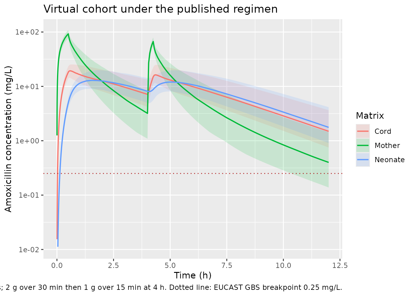
frac_above <- function(conc, time, mic = 0.25, tmax_int = 4) {
  keep <- time <= tmax_int
  conc <- conc[keep]; time <- time[keep]
  above <- conc > mic
  sum(diff(time) * (head(above, -1) & tail(above, -1))) / tmax_int * 100
}

ftmic <- sim_coh |>
  dplyr::group_by(id) |>
  dplyr::summarise(
    Maternal = frac_above(Cc, time),
    Cord     = frac_above(Ccord, time),
    Neonatal = frac_above(Cneonate, time),
    cmax_mat = max(Cc[time <= 4]),
    .groups = "drop"
  )

ftmic_summary <- ftmic |>
  dplyr::select(Maternal, Cord, Neonatal) |>
  tidyr::pivot_longer(everything(), names_to = "Matrix",
                      values_to = "pct") |>
  dplyr::group_by(Matrix) |>
  dplyr::summarise(median = median(pct),
                   q10 = quantile(pct, 0.10),
                   q90 = quantile(pct, 0.90), .groups = "drop")

stopifnot(
  # Cohort-derived, so asserted on the centre and a robust lower
  # quantile rather than on the per-subject minimum (which is not
  # reproducible across rxode2 builds / thread counts).
  all(ftmic_summary$median > 90),
  all(ftmic_summary$q10 > 90),
  # Median maternal Cmax must track the typical-value profile closely;
  # the eta on CL and V1 is modest (CV 28% and 20% on the log scale).
  abs(median(ftmic$cmax_mat) / peaks["Maternal", "cmax"] - 1) < 0.10
)

ftmic_summary |>
  dplyr::mutate(across(c(median, q10, q90), \(x) signif(x, 4))) |>
  dplyr::rename("Matrix" = Matrix,
                "Median %T > 0.25 mg/L" = median,
                "10th percentile" = q10,
                "90th percentile" = q90) |>
knitr::kable()| Matrix | Median %T > 0.25 mg/L | 10th percentile | 90th percentile |
|---|---|---|---|
| Cord | 99.35 | 99.30 | 99.35 |
| Maternal | 99.95 | 99.95 | 99.95 |
| Neonatal | 96.75 | 96.65 | 96.85 |
All three matrices exceed the breakpoint for more than 90% of the 4-h dosing interval, reproducing the paper’s conclusion that “in a first approximation, the 2-g infusion to the mother appears to be adequate for the prevention of group B streptococcal disease”.
Assumptions and deviations
The published Figure 4 and the simulated peak concentrations quoted in Results cannot be reproduced from Table 2. This is the most important caveat for a user of this model, and it is a property of the source, not of the transcription. Three lines of evidence:
-
Terminal slope. Digitised from Figure 4, the maternal curve
falls from its 88.7 mg/L peak at 0.5 h to the 0.01 mg/L axis floor at
roughly 9.4 h – about 3.95 log10 units in 8.9 h, a terminal half-life
near 0.68 h. The slowest eigenvalue of the rate matrix built from Table
2 is 0.328 /h, a terminal half-life of 2.11 h. The maternal-only
three-compartment sub-model (dropping
k14/k41) gives 0.832 /h, i.e. 0.83 h, which is close to the figure. Figure 4’s maternal curve therefore behaves as though the fetal compartments returned no drug to the mother. - Curve ordering. In Figure 4 the cord and neonatal curves lie below the maternal curve at every time shown. In any linear system in which the fetal compartments are fed from, and drain more slowly than, the maternal compartment, they must eventually lie above it; the model of Figure 2 crosses over at about 2 h.
- Peak magnitudes. The neonatal peak simulates at 13.2 mg/L against a published 8.0 mg/L (+65%), and the two are reported to become similar at 1.1 h whereas this model crosses at about 2.0 h. The maternal peak (92.2 vs 88.7, +4.0%) and the cord/maternal peak ratio (21.2% vs 18%) are much closer.
Methods, “Simulations” states that the simulations were run in Berkeley Madonna, i.e. in a second implementation separate from the NONMEM fit, and its equations are not published. The model shipped here is the one that was fitted: Figure 2’s structure with Table 2’s estimates, under NONMEM ADVAN5’s amount-based mass-transfer semantics.
Three independent points fix that reading, and each of them argues against the alternative in which the fetal compartments are concentration-driven “sensor” compartments that return no mass to the mother (an alternative that would reproduce Figure 4’s steep, parallel terminal slopes):
- Methods, “PK analysis” states that “the model was implemented in the
NONMEM ADVAN5 subroutine”. ADVAN5 is the general linear
mass-transfer routine; its
K<i><j>are amount-based first-order rate constants, which is what the ODEs above encode. - Discussion paragraph 1 states that the total maternal CL here (19.7 L/h) is lower than the 22.8 L/h of the same authors’ three-compartment PPROM model, and that this “can be explained by the additional route of elimination toward the neonate”. Drug must physically leave the maternal compartment for its apparent clearance to fall; a sensor compartment removes no mass and would leave CL unchanged.
- The flow-balance recovery of the “calculated” volumes V4 = 3.4 L and V5 = 11.9 L above only works for amount-based transfer in the direction Figure 2 draws.
No parameter was adjusted to move the simulation toward the published peaks.
Other deviations and assumptions:
-
IIV correlation not implemented. Results paragraph
3 states that “A correlation between the random parameters for
interindividual variability was found and was accounted for in the
model”, but the off-diagonal covariance between
etalclandetalvcis not reported in Table 2 or anywhere else in the paper. A diagonal OMEGA is used. Simulated cohorts will therefore have a slightly different joint CL / V1 spread than the published model. -
k41andk54share a point estimate, SE and confidence interval. Table 2 gives both as 1.4 (SE 0.31, CI 0.83-2.1) – identical to every printed digit. That is strong evidence they were a single constrained THETA, but the paper never says so. They are encoded here as two separate parameters carrying the same value, which is numerically identical for simulation and leaves the choice open for anyone re-fitting the model. -
V4 and V5 are
fixed(). They are reported without a standard error, were “calculated” rather than estimated, and are scaling constants for the concentration observables only; they do not enter the amount dynamics. -
The gestational-age coefficient is a prose value.
e_ga_vc = 0.042comes from the sentence “An increase in V1 of 4.2% per week was found”, not from a table row, and carries no reported uncertainty. The centring value 36.8 weeks is printed inside the covariate equation itself and agrees with the Table 1 mean amenorrhoea of 36 6/7 (= 36.857) weeks. -
Body mass index is not implemented. It was
significant on V on its own (dOFV = -8.5) but was dropped in favour of
gestational age; no coefficient is reported, so it could not be
implemented even as an alternative. It is recorded in
covariatesDataExcluded. - Arterial cord and neonatal serum share one compartment. This is the authors’ own simplification (Discussion paragraph 3), forced by the small number of neonatal samples. The paper notes the consequence explicitly: “Because elimination from the neonate to the mother was included in the model, the model-predicted neonatal concentrations were slightly lower than the observed concentrations, as seen in Fig. 3.”
-
cord_venousandneonateare declared aspaper_specific_compartments. Neither is a member of a canonical compartment family. They follow the precedent ofFauchet_2015_lopinavir_placental.R(fetal,amniotic) rather than opening a new canonical namespace for maternal-fetal matrices. -
Rate constants keep the paper’s slot-index names
(
k14,k41,k45,k54,k50). The indices refer to Figure 2’s ADVAN5 slots: 1 = maternal central, 4 = venous umbilical cord, 5 = neonate, 0 = eliminated. The mapping is recorded in the model file’scompartmentDataand in the parameter labels. - Cohort covariate distribution is assumed. Gestational age is drawn from a truncated normal matched to the published mean and SD; the paper reports summary statistics only. Race and ethnicity are not reported at all.
- No published NCA to compare against. The paper reports no non-compartmental parameters, so the PKNCA section verifies internal identities (dose recovery, shared terminal slope) rather than reproducing a published table.