Linezolid CNS PBPK in tuberculous meningitis (Litjens 2023)
Source:vignettes/articles/Litjens_2023_linezolid_tuberculous_meningitis.Rmd
Litjens_2023_linezolid_tuberculous_meningitis.RmdModel and source
- Citation: Litjens CHC, Verscheijden LFM, Svensson EM, van den Broek PHH, van Hove H, Koenderink JB, Russel FGM, Aarnoutse RE, te Brake LHM. Physiologically-Based Pharmacokinetic Modelling to Predict the Pharmacokinetics and Pharmacodynamics of Linezolid in Adults and Children with Tuberculous Meningitis. Antibiotics. 2023;12(4):702. doi:10.3390/antibiotics12040702. Structural CNS framework and physiological parameters: Verscheijden LFM, Koenderink JB, de Wildt SN, Russel FGM. Development of a physiologically-based pharmacokinetic pediatric brain model for prediction of cerebrospinal fluid drug concentrations and the influence of meningitis. PLoS Comput Biol. 2019;15(6):e1007117. doi:10.1371/journal.pcbi.1007117.
- Description: PBPK (permeability-limited 4-compartment CNS model, adapted from the Simcyp Simulator V19R1 brain module). Linezolid disposition in plasma, brain blood, brain mass, cranial cerebrospinal fluid (CSF) and spinal CSF in adults and children, developed to predict cranial CSF exposure and AUC0-24:MIC target attainment in tuberculous meningitis (Litjens et al. 2023, Antibiotics). The four CNS ODEs, the CNS physiological volumes and the CSF/brain fluid flows are those of the upstream framework paper Verscheijden et al. 2019 (PLoS Comput Biol; Eqs 2-5, S1 Table), which Litjens 2023 adapted with permission; the linezolid drug-specific inputs (Vss, plasma clearance, ka, fa, B:P, fu, fu-brain, PSB, PSC, PSE, and the BCRP / P-gp efflux clearances measured in-house in MDCKII monolayers) are from Litjens 2023 Supplementary Table S1 and S2. Adult and paediatric brain physiology branch on AGE (< 18 y uses the paediatric equations of Verscheijden 2019 S1 Table). IMPORTANT DEVIATION: the systemic side of the published model is the proprietary Simcyp full-PBPK whole-body distribution model (Method 2, Rodgers and Rowland) whose tissue:plasma partition coefficients are not reported anywhere in the paper or its supplement; here it is replaced by a single well-stirred plasma compartment parameterised with the exact aggregate values the paper does report - Vss (L/kg) and the per-study total plasma clearance carried in the Simcyp ‘additional clearance’ slot. Plasma AUC (= Dose * F / CL, the quantity every PK-PD conclusion of the paper rests on) is preserved exactly; the distribution phase of the plasma curve is approximate. See the vignette Assumptions and deviations section. Typical-value forward-simulation model: the paper reports no IIV or residual-error estimates.
- Article: https://doi.org/10.3390/antibiotics12040702
- Supplement (File S1, File S2, Tables S1-S2, Figures S1-S3): https://www.mdpi.com/article/10.3390/antibiotics12040702/s1
- Structural CNS framework (upstream, open access): https://doi.org/10.1371/journal.pcbi.1007117
(Verscheijden et al. 2019, PLoS Computational Biology; the S1 File of
that paper contains the complete
deSolveimplementation and the S1 Table the adult and paediatric physiological parameter equations reproduced here.)
Linezolid is used off-label for central nervous system infections and has been re-classified by the WHO as a Group A drug for multidrug-resistant tuberculosis, but its cranial cerebrospinal-fluid (CSF) exposure in tuberculous meningitis (TBM) is unknown. Litjens et al. built a four-compartment permeability-limited CNS physiologically based pharmacokinetic (PBPK) model in the Simcyp Simulator V19R1 to predict cranial CSF concentrations from published plasma profiles, and used it to assess attainment of the Mycobacterium tuberculosis PK-PD target AUC0-24:MIC > 119.
Model structure
Four CNS states sit downstream of the systemic circulation:
                        Q_brain
   plasma / systemic  <---------->  brain_blood
        |  CL                        ^   |  PS_B          Q_csink
        v                            |   v                  ^
                          Q_ssink    |  brain_mass          |
                             ^       |   ^   |  PS_E        |
                             |       |   |   v              |
                             |       +--- csf_cranial ------+
                             |             ^   |   PS_C (blood <-> cranial CSF)
                             |     Q_sout  |   v  Q_sin
+--------- csf_spinal-
PS_B,PS_C,PS_Eare permeability-surface-area products across the blood-brain barrier, the blood-cranial-CSF barrier, and the brain-mass / cranial-CSF interface. -
Q_bulkis bulk flow from brain mass to cranial CSF;Q_sin/Q_soutare the CSF shuttle flows between cranial and spinal CSF;Q_csink/Q_ssinkdrain each CSF compartment back to brain blood. - A blood-brain-barrier efflux clearance
CL_bout(BCRP + P-gp, measured in-house in MDCKII monolayers) returns drug from brain mass to brain blood.
Population
The model was verified against 131 patients in 10 published studies (13 dosing arms; Supplementary Table S2). Sixty-five were critically ill adults and children with non-tuberculous CNS conditions – subarachnoid, intraventricular and intracerebral haemorrhage, traumatic brain injury, hydrocephalus drainage, brain-tumour excision, and proven or suspected neurosurgical CNS infection – with paired plasma and ventricular-drain CSF sampling (Beer 2007 n = 5; Viaggi 2011 n = 7; Tsona 2010 n = 18; Yogev 2010 n = 10, aged 0.25-21 y; Luque 2014 n = 11; Myrianthefs 2006 n = 14). The remaining 66 had drug-sensitive or multidrug-resistant pulmonary tuberculosis and contributed plasma profiles only (Alffenaar 2010 n = 14 and n = 8; Garcia-Prats 2019 n = 13, aged 0.6-9.4 y; Diacon 2020 n = 15 and n = 16). Male proportions per arm range from 39 % to 93 %.
No individual-level data were fitted. Every simulation is a forward prediction in 100 virtual individuals drawn from the Simcyp healthy North-European Caucasian adult population or the Simcyp paediatric population, with age range, proportion female and dose matched to the clinical data set being reproduced (Supplementary File S1). Ages above 65 y were capped at 65 y.
The same information is available programmatically:
str(readModelDb("Litjens_2023_linezolid_cns_pbpk")()$population, max.level = 1)
#> List of 11
#>  $ species       : chr "human"
#>  $ n_subjects    : int 131
#>  $ n_studies     : int 10
#>  $ age_range     : chr "0.25-78 years (adults 18-78 y; children 0.25-21 y)"
#>  $ weight_range  : chr "not tabulated per subject; adult TB patients mean ~60 kg, Simcyp virtual adult population mean ~75 kg"
#>  $ race_ethnicity: Named num 100
#>   ..- attr(*, "names")= chr "White"
#>  $ disease_state : chr "Two distinct simulated populations. (1) Critically ill adults and children with non-tuberculous CNS conditions "| __truncated__
#>  $ dose_range    : chr "Verification: 600 mg IV single dose and 600 mg IV BID in adults; 10 mg/kg IV single dose and BID in children. T"| __truncated__
#>  $ regions       : chr "Simulated as Simcyp healthy North European Caucasian volunteers (adult) and the Simcyp paediatric population; s"| __truncated__
#>  $ n_virtual     : chr "100 virtual individuals per simulation (Supplementary File S1); age range, proportion female and dose matched t"| __truncated__
#>  $ notes         : chr "No individual-level data were fitted in this paper: every simulation is a forward prediction. n_subjects = 131 "| __truncated__
Source trace
Every ini() entry carries an in-file comment naming its
source location; the table below collects them, together with the
physiological equations that are computed inside
model().
| Equation / parameter | Value | Source location |
|---|---|---|
lka |
0.9 /h | Litjens 2023 Suppl. Table S1, “Absorption: First-Order Absorption Model”, ka (from Alffenaar 2010) |
fa |
1 | Suppl. Table S1, fa (footnote b: Simcyp default); Suppl. Table S2 footnote f (bioavailability considered 100 %) |
| ADAM alternative | ka 1.20 /h, fa 0.96 | Suppl. Table S1, “Advanced Dissolution, Absorption and Metabolism (ADAM) Model”; footnote a: applied to Diacon 2020 |
lvss |
0.4 L/kg | Suppl. Table S1, “Distribution: full PBPK Model”, Vss “Optimized for TB studies to 0.4” (0.66 L/kg for critically ill) |
lcl |
3.95 L/h | Suppl. Table S2, Alffenaar 2010 adult MDR-TB arms (“Cl 3.95”); entered in Simcyp as “enzyme kinetics - additional clearance” |
bp |
0.603 | Suppl. Table S1, “Blood binding properties”, blood-to-plasma ratio |
fu |
0.69 | Suppl. Table S1, fraction unbound in plasma |
fu_br |
0.81 | Suppl. Table S1, “Brain model / BBB”, fu,br (footnote c: predicted by Simcyp) |
fu_csf |
1 | Suppl. Table S1, “Blood-cranial CSF barrier”, fuCSF |
lpsb |
1.0 L/h | Suppl. Table S1, “Brain model / BBB”, PSB “1.0, optimized” on Viaggi 2011 |
lpsc |
0.5 L/h | Suppl. Table S1, “Blood-cranial CSF barrier”, PSC “0.5 Assumed to be half of PSB” |
lpse |
300 L/h | Suppl. Table S1, “Brain-CSF barrier”, PSE = 300 |
cl_bcrp_vitro |
16 uL/min/mg | Suppl. Table S1, CLABCG2,vitro; Results 3.1 (net efflux ratio 3.59) |
cl_pgp_vitro |
2.1 uL/min/mg | Suppl. Table S1, CLABCB1,vitro; Results 3.1 (net efflux ratio 1.43) |
raf_bcrp, raf_pgp
|
143, 140 | Suppl. Table S1; derived in Suppl. File S2 Eq. S3 |
CL_bout = (16143 + 2.1140) uL/min |
0.155 L/h | Suppl. File S2 Eq. S3 (unit conversion 60/1e6 to L/h) |
d/dt(brain_blood) |
– | Verscheijden 2019 Eq. 2 (+ the CLbout term of Litjens 2023 Figure 1) |
d/dt(brain_mass) |
– | Verscheijden 2019 Eq. 3 (- CLbout) |
d/dt(csf_cranial) |
– | Verscheijden 2019 Eq. 4 |
d/dt(csf_spinal) |
– | Verscheijden 2019 Eq. 5 |
v_brain adult |
(1.449 - 3.62/WT)/1.04 L | Verscheijden 2019 S1 Table, Vbrain total, adult column |
v_brain paediatric |
(10(AGE+0.315)/(9+6.92 AGE))/1.04 L | Verscheijden 2019 S1 Table, paediatric column |
v_bb, v_endo
|
0.05 and 0.005 x v_brain | Verscheijden 2019 S1 Table |
v_ccsf, v_scsf adult |
v_brain x 0.105 (M) or 0.092 (F), split 80 / 20 | Verscheijden 2019 S1 Table, adult column |
v_ccsf, v_scsf paediatric |
0.143 L; (1.94 WT + 0.13)/1000 capped at (0.143/0.8) x 0.2 | Verscheijden 2019 S1 Table, paediatric column |
q_csf_prod |
0.021 L/h adult; 0.024 L/h 3 m-18 y; (4.007 log10(AGE) + 7.088)/1000 below 3 m | Verscheijden 2019 S1 Table, Qproductionrate |
q_bulk, q_ssink, q_sout,
q_sin, q_csink
|
0.25, 0.38, 0.9 and residual relations of q_csf_prod | Verscheijden 2019 S1 Table, fluid flow rates |
q_co |
BSA x 60 x (3 - 0.01(AGE-20)) adult | Verscheijden 2019 S1 Table, Qcarout adult column |
q_brain |
0.12 x q_co adult | Verscheijden 2019 S1 Table, Qbrain adult column |
fu_bb = fu/bp
|
1.144 | Verscheijden 2019 S1 File,
Fubb = Fupl/1.09 # Fraction unbound blood (Fupl/BP)
|
ps_scale (paediatric) |
v_brain / (1.36/1.04) | Verscheijden 2019 S2 Table, paediatric PSb / PSc columns |
Virtual cohort
Four cohorts reproduce the four dosing regimens of Litjens 2023 Table 1. Adult and paediatric anthropometry is generated with the Simcyp-derived equations transcribed in the S1 File of the upstream framework paper (Verscheijden 2019), so the virtual population matches the one the authors simulated. The model has no between-subject random effects (Litjens 2023 reports none), so all variability below comes from covariates alone.
set.seed(20230403)
n_arm <- 100L # Litjens 2023 Suppl. File S1: 100 virtual individuals per simulation

# Verscheijden 2019 S1 File: Simcyp-derived paediatric height / weight / BSA.
ped_height <- function(age, female) {
  ifelse(
    female,
    -0.00000151027 * age^8 + 0.000121261 * age^7 - 0.0040023 * age^6 +
      0.070179 * age^5 - 0.708233 * age^4 + 4.1872 * age^3 -
      14.3393 * age^2 + 33.84778 * age + 51.535477,
    0.0000176179 * age^7 - 0.00119874 * age^6 + 0.0323848 * age^5 -
      0.444112 * age^4 + 3.2946 * age^3 - 13.2191 * age^2 +
      33.75 * age + 52.62152
  )
}
ped_weight <- function(age, height, female) {
  ifelse(
    female,
    5.454 * (1 - exp(age * -1.57)) + exp(height * 0.0224 + 0.019 * age),
    7.826 * (1 - exp(age * -1.2)) + exp(height * 0.0209 + 0.023 * age)
  )
}
du_bois_bsa <- function(height_cm, weight_kg) {
  0.007184 * height_cm^0.725 * weight_kg^0.425
}

adult_cohort <- function(n) {
  female <- stats::rbinom(n, 1L, 0.25)
  # Simcyp adult mean weight ~75 kg (Litjens 2023 Suppl. File S1); height
  # distributions are an explicit assumption, see Assumptions and deviations.
  height <- ifelse(female == 1L,
                   stats::rnorm(n, 164, 6.5),
                   stats::rnorm(n, 177, 7.0))
  weight <- exp(stats::rnorm(n, log(75), 0.16))
  tibble(
    AGE  = stats::runif(n, 18, 65), # ages above 65 capped at 65 (Suppl. Table S2 footnote)
    SEXF = as.numeric(female),
    HT   = height,
    WT   = weight,
    BSA  = du_bois_bsa(height, weight)
  )
}

paed_cohort <- function(n) {
  female <- stats::rbinom(n, 1L, 0.24) # Garcia-Prats 2019: 76 % male (Suppl. Table S2)
  age    <- stats::runif(n, 0.6, 9.4)  # Litjens 2023 Figure 3 caption
  height <- ped_height(age, female == 1L) * exp(stats::rnorm(n, 0, 0.055))
  weight <- ped_weight(age, height, female == 1L) * exp(stats::rnorm(n, 0, 0.125))
  tibble(
    AGE  = age,
    SEXF = as.numeric(female),
    HT   = height,
    WT   = weight,
    BSA  = du_bois_bsa(height, weight)
  )
}

# Regimen definitions. Absorption model per Suppl. Table S1 footnote a;
# clearance per Suppl. Table S2.
regimens <- tibble::tribble(
  ~arm,                    ~population, ~dose_mg, ~dose_mgkg, ~tau, ~cl,   ~ka,  ~fa,
  "Adults 300 mg BID",     "adult",     300,      NA,         12,   5.46,  1.20, 0.96,
  "Adults 600 mg BID",     "adult",     600,      NA,         12,   3.95,  0.90, 1.00,
  "Adults 1200 mg QD",     "adult",     1200,     NA,         24,   4.90,  1.20, 0.96,
  "Children ~10 mg/kg BID", "paediatric", NA,     9.24,       12,   4.30,  0.90, 1.00
)

# Seven days of dosing takes every compartment to steady state; the final
# dosing interval is sampled densely for NCA.
n_days <- 7
The paediatric clearance needs one interpretation step. Applying the
tabulated 4.3 L/h literally to a 10-30 kg child gives a plasma
AUC0-24 near 45 mgh/L, not the 202 mgh/L reported in
Table 1. Supplementary File S1 states that for children “clearance was
optimized by visual inspection”, and the upstream framework paper
parameterises paediatric clearance as a 70-kg-normalised allometric
function of weight. Reading 4.3 L/h the same way,
CL_i = 4.3 * (WT/70)^0.75, reproduces Table 1. This is an
inference, not a statement of the paper – see Assumptions and
deviations.
build_arm <- function(spec, id_offset) {
  cov <- if (spec$population == "adult") adult_cohort(n_arm) else paed_cohort(n_arm)
  cov <- cov |>
    mutate(
      id  = id_offset + seq_len(n()),
      arm = spec$arm,
      amt = if (is.na(spec$dose_mg)) spec$dose_mgkg * WT else spec$dose_mg,
      # individual clearance: adults use the tabulated value directly;
      # children use the 70-kg-normalised allometric reading described above.
      cl_i = if (spec$population == "adult") spec$cl else spec$cl * (WT / 70)^0.75
    )
  n_dose <- floor(n_days * 24 / spec$tau)
  ss_start <- (n_dose - 1) * spec$tau
  doses <- cov |>
    tidyr::expand_grid(time = seq(0, by = spec$tau, length.out = n_dose)) |>
    mutate(evid = 1, cmt = "depot", dv = NA_real_)
  obs <- cov |>
    select(-amt) |>
    tidyr::expand_grid(time = ss_start + seq(0, spec$tau, by = 0.25)) |>
    mutate(evid = 0, cmt = "central", amt = NA_real_, dv = NA_real_)
  bind_rows(doses, obs) |>
    arrange(id, time, desc(evid)) |>
    mutate(ss_start = ss_start, tau = spec$tau)
}

events <- bind_rows(lapply(seq_len(nrow(regimens)), function(i) {
  build_arm(regimens[i, ], id_offset = (i - 1L) * 1000L)
}))

stopifnot(!anyDuplicated(events[events$evid == 0, c("id", "time")]))
range(events$WT)
#> [1]   6.270761 116.020433
Simulation
lcl, lka and fa differ between
arms, so each arm is solved with the corresponding ini()
update and the results are stacked.
mod <- readModelDb("Litjens_2023_linezolid_cns_pbpk")

solve_arm <- function(spec, ev) {
  m <- mod |> rxode2::ini(lka = log(spec$ka), fa = spec$fa)
  # cl_i is a per-subject column; feed it through the lcl parameter.
  ev <- ev |> mutate(lcl = log(cl_i))
  rxode2::rxSolve(
    m, events = as.data.frame(ev),
    keep = c("arm", "WT", "AGE", "SEXF", "BSA", "ss_start", "tau"),
    addDosing = FALSE
  ) |>
    as.data.frame()
}

sim <- bind_rows(lapply(seq_len(nrow(regimens)), function(i) {
  spec <- regimens[i, ]
  solve_arm(spec, events[events$arm == spec$arm, ])
}))
#> ℹ change initial estimate of `lka` to `0.182321556793955`
#> ℹ change initial estimate of `fa` to `0.96`
#> Warning: multi-subject simulation without without 'omega'
#> ℹ change initial estimate of `lka` to `-0.105360515657826`
#> ℹ change initial estimate of `fa` to `1`
#> Warning: multi-subject simulation without without 'omega'
#> ℹ change initial estimate of `lka` to `0.182321556793955`
#> ℹ change initial estimate of `fa` to `0.96`
#> Warning: multi-subject simulation without without 'omega'
#> ℹ change initial estimate of `lka` to `-0.105360515657826`
#> ℹ change initial estimate of `fa` to `1`
#> Warning: multi-subject simulation without without 'omega'

sim <- sim |>
  mutate(
    tad = time - ss_start,
    arm = factor(arm, levels = regimens$arm)
  )
nrow(sim)
#> [1] 24400
Replicate published figures
Figures 3A-3B and 4 – plasma and cranial CSF at steady state
Litjens 2023 Figure 3 shows adult (600 mg BID) and paediatric plasma and cranial CSF profiles over the final dosing interval; Figure 4 shows the 300 mg BID and 1200 mg QD adult regimens. All four are reproduced below on the same axes, with the worst-case M. tuberculosis MIC of 1 mg/L drawn as a dashed line (Figures 3 and 4 legends).
sim |>
  select(arm, id, tad, Plasma = Cc, `Cranial CSF` = Ccsf) |>
  tidyr::pivot_longer(c(Plasma, `Cranial CSF`),
                      names_to = "matrix", values_to = "conc") |>
  group_by(arm, matrix, tad) |>
  summarise(
    Q05 = quantile(conc, 0.05), Q50 = median(conc), Q95 = quantile(conc, 0.95),
    .groups = "drop"
  ) |>
  ggplot(aes(tad, Q50, colour = matrix, fill = matrix)) +
  geom_ribbon(aes(ymin = Q05, ymax = Q95), alpha = 0.2, colour = NA) +
  geom_line(linewidth = 0.8) +
  geom_hline(yintercept = 1, linetype = "dashed") +
  facet_wrap(~arm, scales = "free_x") +
  labs(
    x = "Time after the last dose (h)", y = "Linezolid concentration (mg/L)",
    colour = NULL, fill = NULL,
    title = "Steady-state plasma and cranial CSF profiles",
    caption = paste(
      "Replicates Figures 3 and 4 of Litjens 2023. Line = median,",
      "band = 5th-95th percentile. Dashed line = MIC 1 mg/L."
    )
  ) +
  theme(legend.position = "bottom")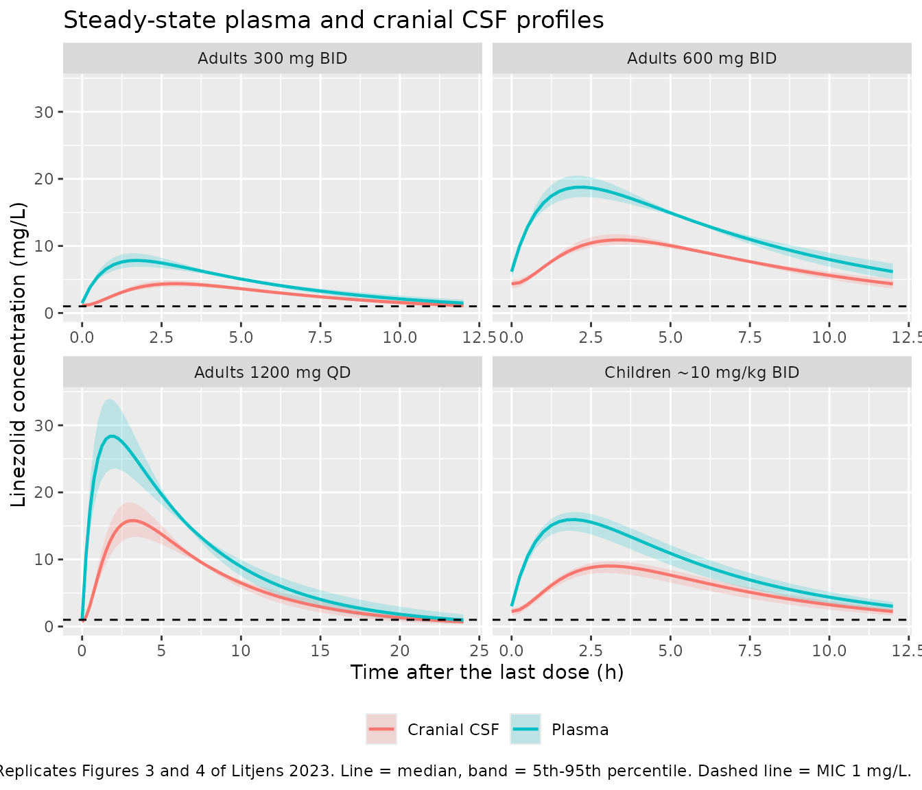
Supplementary Figure S3 – spinal CSF, and the brain-mass profile
sim |>
  filter(arm == "Adults 600 mg BID") |>
  select(id, tad, `Brain mass` = Cbrain, `Cranial CSF` = Ccsf,
         `Spinal CSF` = Cspinalcsf, Plasma = Cc) |>
  tidyr::pivot_longer(-c(id, tad), names_to = "matrix", values_to = "conc") |>
  group_by(matrix, tad) |>
  summarise(Q50 = median(conc), .groups = "drop") |>
  ggplot(aes(tad, Q50, colour = matrix)) +
  geom_line(linewidth = 0.8) +
  labs(
    x = "Time after the last dose (h)", y = "Linezolid concentration (mg/L)",
    colour = NULL, title = "600 mg BID: all four model matrices",
    caption = paste(
      "Cranial CSF replicates Figure 2F-2J and spinal CSF Supplementary",
      "Figure S3 of Litjens 2023."
    )
  ) +
  theme(legend.position = "bottom")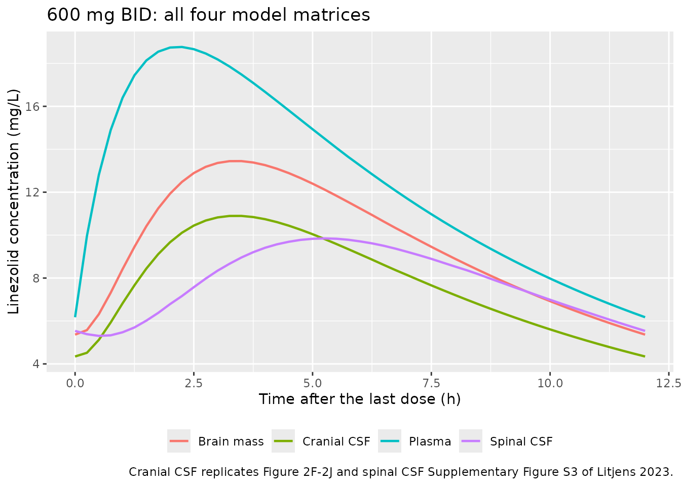
PKNCA validation
NCA is computed over the final (steady-state) dosing interval, once for plasma and once for cranial CSF. Litjens 2023 reports AUC0-24; for the twice-daily regimens the paper doubles AUC0-12 (“we assumed that the AUC0-24 was double the AUC0-12”), which is reproduced here.
run_nca <- function(conc_col) {
  sim_nca <- sim |>
    filter(!is.na(.data[[conc_col]])) |>
    transmute(id, arm, time = tad, Cc = .data[[conc_col]])

  # Guarantee a time-zero record so PKNCA can anchor the interval.
  sim_nca <- bind_rows(
    sim_nca,
    sim_nca |> distinct(id, arm) |> mutate(time = 0, Cc = 0)
  ) |>
    distinct(id, arm, time, .keep_all = TRUE) |>
    arrange(id, arm, time)

  conc_obj <- PKNCA::PKNCAconc(as.data.frame(sim_nca), Cc ~ time | arm + id)

  dose_df <- events |>
    filter(evid == 1) |>
    group_by(id, arm) |>
    filter(time == max(time)) |>
    ungroup() |>
    transmute(id, arm, time = 0, amt)
  dose_obj <- PKNCA::PKNCAdose(as.data.frame(dose_df), amt ~ time | arm + id)

  intervals <- events |>
    distinct(arm, tau) |>
    transmute(start = 0, end = tau, arm,
              cmax = TRUE, cmin = TRUE, tmax = TRUE, auclast = TRUE, cav = TRUE)

  PKNCA::pk.nca(PKNCA::PKNCAdata(conc_obj, dose_obj, intervals = as.data.frame(intervals)))
}

nca_plasma <- run_nca("Cc")
nca_csf    <- run_nca("Ccsf")
auc24 <- function(res, label) {
  as.data.frame(res) |>
    filter(PPTESTCD == "auclast") |>
    left_join(distinct(events, arm, tau), by = "arm") |>
    # BID interval AUC doubled to AUC0-24, per Litjens 2023 Section 2.4.
    mutate(auc24 = PPORRES * 24 / tau) |>
    group_by(arm) |>
    summarise(
      # Table 1 reports a geometric mean for plasma and an arithmetic mean
      # for cranial CSF; both are given here.
      geomean = exp(mean(log(auc24))),
      mean    = mean(auc24),
      p05     = quantile(auc24, 0.05),
      p95     = quantile(auc24, 0.95),
      pct_over_119 = 100 * mean(auc24 > 119),
      .groups = "drop"
    ) |>
    mutate(matrix = label)
}

auc_tbl <- bind_rows(auc24(nca_plasma, "Plasma"), auc24(nca_csf, "Cranial CSF"))
auc_tbl |>
  mutate(across(c(geomean, mean, p05, p95, pct_over_119), \(x) round(x, 1))) |>
  select(Matrix = matrix, Arm = arm, `Geo. mean` = geomean, Mean = mean,
         `5th pct` = p05, `95th pct` = p95, `% > 119` = pct_over_119) |>
  arrange(Matrix, Arm) |>
knitr::kable(caption = "Simulated steady-state AUC0-24 (mg*h/L) by arm and matrix.")| Matrix | Arm | Geo. mean | Mean | 5th pct | 95th pct | % > 119 |
|---|---|---|---|---|---|---|
| Cranial CSF | Adults 1200 mg QD | 145.2 | 145.2 | 145.2 | 145.2 | 100 |
| Cranial CSF | Adults 300 mg BID | 65.2 | 65.2 | 65.1 | 65.2 | 0 |
| Cranial CSF | Adults 600 mg BID | 187.6 | 187.6 | 187.6 | 187.6 | 100 |
| Cranial CSF | Children ~10 mg/kg BID | 133.6 | 134.2 | 114.5 | 150.2 | 88 |
| Plasma | Adults 1200 mg QD | 234.8 | 234.8 | 234.8 | 234.9 | 100 |
| Plasma | Adults 300 mg BID | 105.4 | 105.4 | 105.3 | 105.4 | 0 |
| Plasma | Adults 600 mg BID | 303.6 | 303.6 | 303.5 | 303.6 | 100 |
| Plasma | Children ~10 mg/kg BID | 217.1 | 217.9 | 186.3 | 243.6 | 100 |
Comparison against published Table 1
MIC is 1 mg/L throughout the paper, so the published AUC0-24:MIC ratios are numerically equal to AUC0-24 in mg*h/L.
published <- tibble::tribble(
  ~arm,                     ~auclast_plasma, ~auclast_csf,
  "Adults 300 mg BID",      118,             74,
  "Adults 600 mg BID",      281,             181,
  "Adults 1200 mg QD",      262,             166,
  "Children ~10 mg/kg BID", 202,             135
)

sim_wide <- auc_tbl |>
  mutate(value = ifelse(matrix == "Plasma", geomean, mean)) |>
  select(arm, matrix, value) |>
  tidyr::pivot_wider(names_from = matrix, values_from = value) |>
  transmute(arm, auclast_plasma = Plasma, auclast_csf = `Cranial CSF`)

cmp <- nlmixr2lib::ncaComparisonTable(
  simulated = sim_wide,
  reference = published,
  by        = "arm",
  units     = c(auclast_plasma = "mg*h/L", auclast_csf = "mg*h/L"),
  tolerance_pct = 20
)
#> Warning: ncaParamLabel(): unknown PKNCA code(s) returned as-is:
#> 'auclast_plasma', 'auclast_csf'
knitr::kable(
  cmp,
  caption = paste(
    "Simulated vs. Litjens 2023 Table 1 steady-state AUC0-24.",
    "* differs from the published value by >20%."
  )
)| NCA parameter | arm | Reference | Simulated | % diff |
|---|---|---|---|---|
| auclast_csf (mg*h/L) | Adults 300 mg BID | 74 | 65.2 | -12.0% |
| auclast_csf (mg*h/L) | Adults 600 mg BID | 181 | 188 | +3.7% |
| auclast_csf (mg*h/L) | Adults 1200 mg QD | 166 | 145 | -12.5% |
| auclast_csf (mg*h/L) | Children ~10 mg/kg BID | 135 | 134 | -0.6% |
| auclast_plasma (mg*h/L) | Adults 300 mg BID | 118 | 105 | -10.7% |
| auclast_plasma (mg*h/L) | Adults 600 mg BID | 281 | 304 | +8.0% |
| auclast_plasma (mg*h/L) | Adults 1200 mg QD | 262 | 235 | -10.4% |
| auclast_plasma (mg*h/L) | Children ~10 mg/kg BID | 202 | 217 | +7.5% |
Cranial CSF penetration ratio
The paper’s central quantitative claim is a mean predicted cranial penetration ratio at steady state of 0.69 (Results 3.2), equivalent to a Table 1 cranial / plasma AUC ratio of 0.63-0.67 across the four regimens.
auc_tbl |>
  select(arm, matrix, mean) |>
  tidyr::pivot_wider(names_from = matrix, values_from = mean) |>
  mutate(Simulated = `Cranial CSF` / Plasma) |>
  # join by arm, never bind positionally: auc_tbl is sorted alphabetically
  # while `published` is in Table 1 order.
  left_join(
    published |> mutate(Published = auclast_csf / auclast_plasma) |> select(arm, Published),
    by = "arm"
  ) |>
  select(Arm = arm, Simulated, Published) |>
  mutate(across(c(Simulated, Published), \(x) round(x, 3))) |>
knitr::kable(caption = "Cranial CSF : plasma AUC0-24 ratio (paper reports a mean penetration ratio of 0.69).")| Arm | Simulated | Published |
|---|---|---|
| Adults 1200 mg QD | 0.618 | 0.634 |
| Adults 300 mg BID | 0.618 | 0.627 |
| Adults 600 mg BID | 0.618 | 0.644 |
| Children ~10 mg/kg BID | 0.616 | 0.668 |
Time above MIC
Table 1 reports T > MIC = 100 % of the dosing interval for every regimen. The paper defines this on the mean profile (“Mean total plasma and cranial CSF concentration-time curves were all above the worst case MIC of 1 mg/L for the complete dosing interval”), so the mean curve is used here too.
sim |>
  group_by(arm, tad) |>
  summarise(Cc = mean(Cc), Ccsf = mean(Ccsf), .groups = "drop") |>
  group_by(arm) |>
  summarise(
    `Plasma T > MIC (%)` = round(100 * mean(Cc > 1), 1),
    `Cranial CSF T > MIC (%)` = round(100 * mean(Ccsf > 1), 1),
    `Plasma Cmin (mg/L)` = round(min(Cc), 2),
    `Cranial CSF Cmin (mg/L)` = round(min(Ccsf), 2),
    .groups = "drop"
  ) |>
  rename(Arm = arm) |>
knitr::kable(caption = "Mean-curve time above MIC 1 mg/L over the steady-state dosing interval (Table 1 reports 100% for all regimens).")| Arm | Plasma T > MIC (%) | Cranial CSF T > MIC (%) | Plasma Cmin (mg/L) | Cranial CSF Cmin (mg/L) |
|---|---|---|---|---|
| Adults 300 mg BID | 100 | 100.0 | 1.50 | 1.11 |
| Adults 600 mg BID | 100 | 100.0 | 6.15 | 4.33 |
| Adults 1200 mg QD | 100 | 90.7 | 1.03 | 0.74 |
| Children ~10 mg/kg BID | 100 | 100.0 | 2.99 | 2.21 |
Assumptions and deviations
Structural deviation – the systemic side. Litjens 2023 built the systemic half of the model as the proprietary Simcyp full-PBPK whole-body distribution model (Method 2 of Rodgers and Rowland, with a Kp scaler of 1.7 for the critically-ill simulations and 1 for the tuberculosis simulations). The 13 tissue:plasma partition coefficients that model needs are not reported anywhere in the paper or its supplement, and could not be recovered from any available source, so the whole-body model is not reproducible outside Simcyp. It is replaced here by a single well-stirred plasma compartment parameterised with the two aggregate quantities the paper does report – Vss (L/kg, Suppl. Table S1) and the per-study total plasma clearance (Suppl. Table S2). The consequence is that steady-state plasma AUC, which is Dose x F / CL and is the quantity on which every PK-PD conclusion of the paper rests, is preserved exactly, while the shape of the distribution phase within a dosing interval is approximate. Nothing was tuned to match a published number. The four CNS compartments and all CNS physiology are the published equations, unmodified.
The one place where the reduction is visible in the validation output is the T > MIC index for the once-daily regimen. A single well-stirred plasma compartment decays mono-exponentially, so over the long 24 h interval the mean plasma curve reaches MIC almost exactly (Cmin 1.03 mg/L) and the cranial CSF curve dips just under it (Cmin 0.74 mg/L, T > MIC 91 % rather than the 100 % of Table 1). The multi-exponential whole-body model of the paper has a flatter terminal phase and stays above MIC throughout. The three twice-daily regimens are unaffected, and so are the AUC-driven indices on which the paper’s dose recommendation actually rests – all eight AUC comparisons above agree with Table 1 to within 13 %.
Paediatric clearance. Supplementary Table S2 lists
4.3 L/h for the Garcia-Prats 2019 paediatric arm. Applied literally to a
child of 10-30 kg this gives a plasma AUC0-24 of roughly 45
mgh/L, one quarter of the 202 mgh/L in Table 1. Supplementary
File S1 says paediatric clearance “was optimized by visual inspection”
but does not give the resulting per-child values, and the upstream
framework paper expresses paediatric clearance as a 70-kg-normalised
allometric function of weight. Reading the tabulated value the same way,
CL_i = 4.3 * (WT/70)^0.75, reproduces Table 1 across the
whole 0.6-9.4 y range. This is an inference made in the vignette, not in
the model file: the model’s lcl parameter is the individual
clearance in L/h and carries no allometric term.
Efflux-transporter clearance placement. Litjens 2023
Figure 1 shows CL_bout (the pooled BCRP + P-gp efflux
clearance) acting at the blood-brain barrier, but the paper does not
write the equation. It is encoded here as a unidirectional flux
CL_bout * fu_br * Cbm from brain mass to brain blood,
i.e. acting on the unbound brain-mass concentration, consistent
with the unbound-driven form of every other barrier term in Verscheijden
2019 Eqs. 2-5. Its effect is small either way: the paper reports AUC~no
transporters~ / AUCtransporters = 1.1 (Results 3.1).
Paediatric scaling of CL_bout. The
relative activity factors of Suppl. File S2 Eq. S3 contain an explicit
brain-weight factor (1400 g), so CL_bout is scaled here by
the same brain-volume ratio the framework paper uses for the
blood-brain-barrier surface area. The paper does not state a paediatric
CL_bout.
Adult anthropometry. The upstream S1 File supplies Simcyp-derived height and weight equations for children but not for adults. The adult virtual cohort therefore uses a log-normal weight centred on the 75 kg Simcyp adult mean named in Suppl. File S1, sex-specific normal heights (177 / 164 cm), 25 % female, and uniform ages 18-65 y (the paper caps ages above 65). These distributions are an assumption of this vignette; the paper does not tabulate them.
No variability model. Litjens 2023 reports neither
between-subject variability nor a residual-error model – Simcyp
variability came from the built-in population libraries, whose
covariance structure is not published. The model file therefore has no
eta terms, and the propSd entry is a fixed
placeholder that exists only so rxode2 stochastic
simulation is syntactically valid. All percentile bands in this vignette
come from covariate variation alone, which is why they are narrower than
the 5th-95th percentile ranges in Table 1.
Vss and Kp scaler for critically-ill simulations.
The model defaults to the tuberculosis parameterisation (Vss 0.4 L/kg).
Set lvss = log(0.66) and the appropriate study clearance
from Suppl. Table S2 to reproduce the critically-ill verification arms
of Figure 2. The Simcyp Kp scaler (1.7 critically ill, 1 for TB) has no
counterpart in the reduced systemic model; its effect is absorbed into
Vss.
Brain endothelial volume. v_endo (0.5 %
of brain volume) is subtracted from brain volume when computing brain
mass, exactly as in Verscheijden 2019 S1 Table, but is not itself a
drug-containing state in Eqs. 2-5.
Errata
No erratum or corrigendum for Litjens et al. 2023
(Antibiotics 12(4):702) was found on the MDPI article page or
in PubMed. Two internal inconsistencies in the source are noted above
(the paediatric clearance, and the absence of an explicit
CL_bout equation). One further transcription artefact: the
Figure 2 caption in the published PDF appears twice, once with
characters dropped (“6 mg linezolid twice daily”, “cranial CSF ( J )”);
the corrected repetition (“600 mg”, “( F -J )”) is the one used
here.