Extended-release injectable olanzapine TV-44749 and oral olanzapine (Perlstein 2026)
Source:vignettes/articles/Perlstein_2026_olanzapine.Rmd
Perlstein_2026_olanzapine.RmdModels and source
This paper developed two population PK models from one Phase 1 study, fitted to two separate datasets, and both are packaged here:
mod_lai  <- readModelDb("Perlstein_2026_olanzapine_lai")
mod_oral <- readModelDb("Perlstein_2026_olanzapine_oral")
ui_lai   <- rxode2::rxode(mod_lai)
#> ℹ parameter labels from comments will be replaced by 'label()'
ui_oral  <- rxode2::rxode(mod_oral)
#> ℹ parameter labels from comments will be replaced by 'label()'-
Perlstein_2026_olanzapine_lai— Two-compartment population PK model for olanzapine following subcutaneous TV-44749, an extended-release copolymer-based long-acting injectable, in adults with schizophrenia or schizoaffective disorder and in healthy participants (Perlstein 2026). Absorption is a convolution-based prescribed input function: a double Weibull release profile splitting the dose between a rapid first release process and a delayed sustained second release process, implemented as two parallel depot compartments each emptying with its own Weibull hazard. Allometric body weight on CL/F and V/F with estimated exponents, and a linear dose effect on the second-process release time. Carries the published Emax dopamine D2 receptor occupancy layer (Mamo 2008) as an algebraic observable. -
Perlstein_2026_olanzapine_oral— Two-compartment population PK model for oral olanzapine (ZYPREXA tablets) with first-order absorption and an absorption lag time, in healthy participants and adults with schizophrenia or schizoaffective disorder (Perlstein 2026). Companion oral comparator model to the TV-44749 subcutaneous long-acting injectable model Perlstein_2026_olanzapine_lai; the two were fitted to separate datasets in the same Phase 1 study. No covariates were retained. Carries the published Emax dopamine D2 receptor occupancy layer (Mamo 2008) as an algebraic observable. - Citation: Perlstein I, Cherniakov I, Elgart A, Gomeni R, Gutman D, Merenlender Wagner A, Singh R. Population Pharmacokinetic Model-Based Dose Selection of Extended-Release Injectable Olanzapine (TV-44749) for Subcutaneous Use in Phase 3 Clinical Trial in Adults with Schizophrenia. The Journal of Clinical Pharmacology. 2026;66(1):e70144. doi:10.1002/jcph.70144. D2 receptor occupancy layer from Mamo D, Kapur S, Keshavan M, et al. D2 receptor occupancy of olanzapine pamoate depot using positron emission tomography: an open-label study in patients with schizophrenia. Neuropsychopharmacology. 2008;33(2):298-304.
- Article: https://doi.org/10.1002/jcph.70144
- Supplement: the Supplementary Online Material PDF, whose Supplemental Table 2 holds the complete oral olanzapine parameter set. The main text never cites Table S2 by number — it references only Table S1 (demographics) and Figure S2 (VPC) — so the oral model is easy to miss.
TV-44749 is an investigational once-monthly subcutaneous long-acting injectable olanzapine built on a copolymer delivery technology: the copolymer precipitates on injection, forming a depot that entraps olanzapine and releases it over the monthly interval. The analysis exists to pick Phase 3 doses that match approved oral olanzapine exposure and land dopamine D2 receptor occupancy (D2RO) in the 60%-80% therapeutic window.
Population
89 participants contributed 3530 olanzapine plasma samples to the TV-44749 model and 90 participants contributed 1196 samples to the oral model, all from the single Phase 1 study TV-44749-SAD-10154. The cohort was 18-60 years (healthy participants) and 18-65 years (patients); cohort mean 45.6 years (SD 10.3), mean weight 85.8 kg (SD 15.7), mean BMI 28.3 kg/m^2 (SD 4.7), 73% male, 79% Black or African American and 69% smokers (Results, Data; per-cohort detail in Supplemental Table 1).
Healthy participants received subtherapeutic single TV-44749 doses (70 or 105 mg); patients with schizophrenia or schizoaffective disorder received single doses of 318, 425 or 531 mg or three consecutive monthly doses of 283 or 566 mg. Every participant took daily oral olanzapine before the injection period, which is what supports the oral model.
The same information is available programmatically via
rxode2::rxode(readModelDb("Perlstein_2026_olanzapine_lai"))$population.
Source trace
Every ini() entry in both model files carries an in-file
comment naming its source location. Collected here for review.
TV-44749 (Perlstein_2026_olanzapine_lai)
| Equation / parameter | Value | Source location |
|---|---|---|
Release function
r(t) = FF*exp(-(t/TD)^SS) + (1-FF)*exp(-(t/TD1)^SS1)
|
n/a | Methods p. 4, unnumbered display equation; Figure 2a |
Disposition ODEs dA1/dt, dA2/dt,
Cp = A1/(V/F)
|
n/a | Methods p. 4, unnumbered display equations |
lra (paper TD) |
117 h, encoded log(1/117)
|
Table 1, Fixed effect |
lgam1 (paper SS) |
1.4 | Table 1, Fixed effect |
lra2 (paper TD1_0) |
323 h, encoded log(1/323)
|
Table 1, Fixed effect |
lgam2 (paper SS1) |
3.25 | Table 1, Fixed effect |
logitfrel (paper FF) |
0.236 | Table 1, Fixed effect |
lcl (CL/F) |
16.6 L/h | Table 1, Fixed effect |
lvc (V/F) |
15.4 L | Table 1, Fixed effect |
lk12 |
1.61 1/h | Table 1, Fixed effect |
lk21 |
0.00313 1/h | Table 1, Fixed effect |
e_wt_cl (CL_P) |
0.31 | Table 1, Fixed effect |
e_wt_vc (V_P) |
0.364 | Table 1, Fixed effect |
e_dose_ra2 (TD1_1) |
0.0939 h/mg | Table 1, Fixed effect; footnote defines TD1_0 /
TD1_1
|
| IIV on all nine structural parameters | 0.0038 - 0.445 | Table 1, Random effect |
addSd / propSd
|
0.632 / 0.233 | Table 1, Fixed effect (“Additive / Proportional RSE model”) |
emax (ROmax) |
100% (fixed) | Methods, PK/D2RO Model (Mamo 2008) |
lec50 (EC50) |
11 ng/mL (fixed) | Methods, PK/D2RO Model (Mamo 2008) |
Oral olanzapine (Perlstein_2026_olanzapine_oral)
| Equation / parameter | Value | Source location |
|---|---|---|
| Two-compartment, first-order absorption with lag | n/a | Methods p. 4 and Figure 2b |
lka |
0.0292 1/h | Supplemental Table 2 |
lvc |
9.61 L | Supplemental Table 2 |
lcl |
22.6 L/h | Supplemental Table 2 |
lk12 / lk21
|
0.254 / 0.015 1/h | Supplemental Table 2 |
ltlag |
0.937 h | Supplemental Table 2 |
| IIV on ka, V/F, CL/F | 0.0444 / 0.897 / 0.227 | Supplemental Table 2, Random-effect |
| No IIV on k12, k21 | n/a | Supplemental Table 2 footnote (“The IIV of k12 and k21 were fixed to zero”) |
addSd (fixed) / propSd
|
0.0001 / 0.147 | Supplemental Table 2 (* marks the fixed additive
term) |
Virtual cohort
Original observed data are not public. The simulations below follow the paper’s own Monte Carlo design (Methods, Simulations): individual parameters are drawn from the estimated fixed- and random-effect distributions, and body weight is resampled from the analysis-dataset distribution, mean (SD) 85.84 (15.68) kg. The paper simulated 250 participants; 200 per arm is used here, the nlmixr2lib cap.
Eight arms are simulated: five TV-44749 once-monthly doses spanning the paper’s stated dose-proportionality range (283-566 mg), and the three oral daily doses they are meant to match.
rxode2::rxSetSeed(20260824)
set.seed(20260824)

N_PER_ARM <- 200L
TAU_LAI   <- 672    # once-monthly, h
TAU_ORAL  <- 24     # once-daily, h
ND_LAI    <- 35L    # injections simulated before the evaluated interval
ND_ORAL   <- 45L    # daily doses simulated before the evaluated interval

# One weight vector, reused across every arm, so the arms are paired
# (common random numbers) exactly as a matched dose-selection comparison needs.
wt_cohort <- pmax(45, rnorm(N_PER_ARM, mean = 85.84, sd = 15.68))

# TV-44749 is dosed onto TWO parallel depots -- the model splits the injected
# dose between the rapid and the sustained release process via f(depot) and
# f(depot2) -- so each injection needs one dose record per depot.
make_lai_arm <- function(dose_mg, id_offset) {
  ids  <- id_offset + seq_len(N_PER_ARM)
  dose_times <- seq(0, by = TAU_LAI, length.out = ND_LAI)
  dosing <- tidyr::crossing(id = ids, time = dose_times, cmt = c("depot", "depot2")) |>
    mutate(amt = dose_mg, evid = 1L)
  obs <- tidyr::crossing(
    id = ids,
    time = TAU_LAI * (ND_LAI - 1) + seq(0, TAU_LAI, by = 6)
  ) |>
    mutate(amt = NA_real_, evid = 0L, cmt = "central")
  bind_rows(dosing, obs) |>
    mutate(
      WT              = wt_cohort[id - id_offset],
      DOSE_TV44749_MG = dose_mg,
      dose_mg         = dose_mg,
      treatment       = sprintf("TV-44749 %d mg QM", dose_mg)
    ) |>
    arrange(id, time, evid)
}

make_oral_arm <- function(dose_mg, id_offset) {
  ids <- id_offset + seq_len(N_PER_ARM)
  dosing <- tidyr::crossing(id = ids, time = seq(0, by = TAU_ORAL, length.out = ND_ORAL)) |>
    mutate(amt = dose_mg, evid = 1L, cmt = "depot")
  obs <- tidyr::crossing(
    id = ids,
    time = TAU_ORAL * (ND_ORAL - 1) + seq(0, TAU_ORAL, by = 0.5)
  ) |>
    mutate(amt = NA_real_, evid = 0L, cmt = "central")
  bind_rows(dosing, obs) |>
    mutate(
      WT        = wt_cohort[id - id_offset],
      dose_mg   = dose_mg,
      treatment = sprintf("Oral olanzapine %d mg QD", dose_mg)
    ) |>
    arrange(id, time, evid)
}

lai_doses  <- c(283, 318, 425, 531, 566)
oral_doses <- c(10, 15, 20)

ev_lai <- bind_rows(lapply(seq_along(lai_doses), function(i)
  make_lai_arm(lai_doses[i], id_offset = (i - 1L) * N_PER_ARM)))
ev_oral <- bind_rows(lapply(seq_along(oral_doses), function(i)
  make_oral_arm(oral_doses[i], id_offset = 10000L + (i - 1L) * N_PER_ARM)))

# Disjoint IDs across arms are mandatory: rxSolve treats id as the subject key
# and would silently merge colliding ids into one over-dosed subject. Note the
# frame is NOT wrapped in unique() -- that would strip the very duplicate rows
# the assertion tests for, leaving a check that can never go red.
stopifnot(
  !anyDuplicated(ev_lai[, c("id", "time", "evid", "cmt")]),
  !anyDuplicated(ev_oral[, c("id", "time", "evid", "cmt")]),
  length(intersect(ev_lai$id, ev_oral$id)) == 0L
)
Both regimens are simulated well past steady state. The TV-44749
model carries a deep peripheral compartment (k21 = 0.00313
1/h, with 74% CV), so a minority of simulated subjects approach steady
state only slowly — the slowest eta draws have terminal half-lives of
several months. Thirty-five monthly injections brings the 5th percentile
of the mass-balance check below to within 1% of its asymptotic value of
1 (see the steady-state identity below).
Simulation
sim_lai <- rxode2::rxSolve(
  mod_lai, events = ev_lai, keep = c("treatment", "dose_mg", "WT")
) |> as.data.frame()
#> ℹ parameter labels from comments will be replaced by 'label()'

sim_oral <- rxode2::rxSolve(
  mod_oral, events = ev_oral, keep = c("treatment", "dose_mg", "WT")
) |> as.data.frame()
#> ℹ parameter labels from comments will be replaced by 'label()'

stopifnot(!anyNA(sim_lai$Cc), !anyNA(sim_oral$Cc),
          all(sim_lai$Cc >= 0), all(sim_oral$Cc >= 0))

# Time relative to the start of the evaluated (final) dosing interval.
sim_lai$trel  <- sim_lai$time  - TAU_LAI  * (ND_LAI  - 1)
sim_oral$trel <- sim_oral$time - TAU_ORAL * (ND_ORAL - 1)
Replicate published figures
Figure 4 — steady-state concentration-time profiles
Figure 4 of Perlstein 2026 overlays the median steady-state olanzapine profile after subcutaneous TV-44749 against the sawtooth profile of daily oral olanzapine, with 90% prediction intervals. Reproduced here for the three selected dose pairs. The oral arms are tiled across the 28-day window so both formulations share one time axis.
sel_pairs <- tibble::tribble(
  ~lai_dose, ~oral_dose, ~pair,
  318L, 10L, "TV-44749 318 mg QM vs oral 10 mg QD",
  425L, 15L, "TV-44749 425 mg QM vs oral 15 mg QD",
  531L, 20L, "TV-44749 531 mg QM vs oral 20 mg QD"
)

quant_by <- function(d, group_cols) {
  d |>
    group_by(across(all_of(group_cols))) |>
    summarise(
      Q05 = quantile(Cc, 0.05), Q50 = median(Cc), Q95 = quantile(Cc, 0.95),
      .groups = "drop"
    )
}

lai_band <- sim_lai |>
  filter(dose_mg %in% sel_pairs$lai_dose) |>
  quant_by(c("dose_mg", "trel")) |>
  left_join(sel_pairs, by = c("dose_mg" = "lai_dose")) |>
  mutate(formulation = "TV-44749 SC (QM)")

# Tile the 24 h oral profile across the 28-day TV-44749 window.
oral_band <- sim_oral |>
  quant_by(c("dose_mg", "trel")) |>
  left_join(sel_pairs, by = c("dose_mg" = "oral_dose")) |>
  tidyr::crossing(day = 0:27) |>
  mutate(trel = trel + day * 24, formulation = "Oral olanzapine (QD)") |>
  filter(trel <= TAU_LAI)

bind_rows(lai_band, oral_band) |>
  ggplot(aes(trel / 24, Q50, colour = formulation, fill = formulation)) +
  geom_ribbon(aes(ymin = Q05, ymax = Q95), alpha = 0.18, colour = NA) +
  geom_line(linewidth = 0.6) +
  facet_wrap(~pair, ncol = 1) +
  labs(
    x = "Time within the dosing interval (days)",
    y = "Olanzapine plasma concentration (ng/mL)",
    colour = NULL, fill = NULL,
    title = "Figure 4 - steady-state profiles, TV-44749 vs oral olanzapine",
    caption = "Replicates Figure 4 of Perlstein 2026. Lines are medians, bands the 90% prediction interval."
  ) +
  theme(legend.position = "bottom")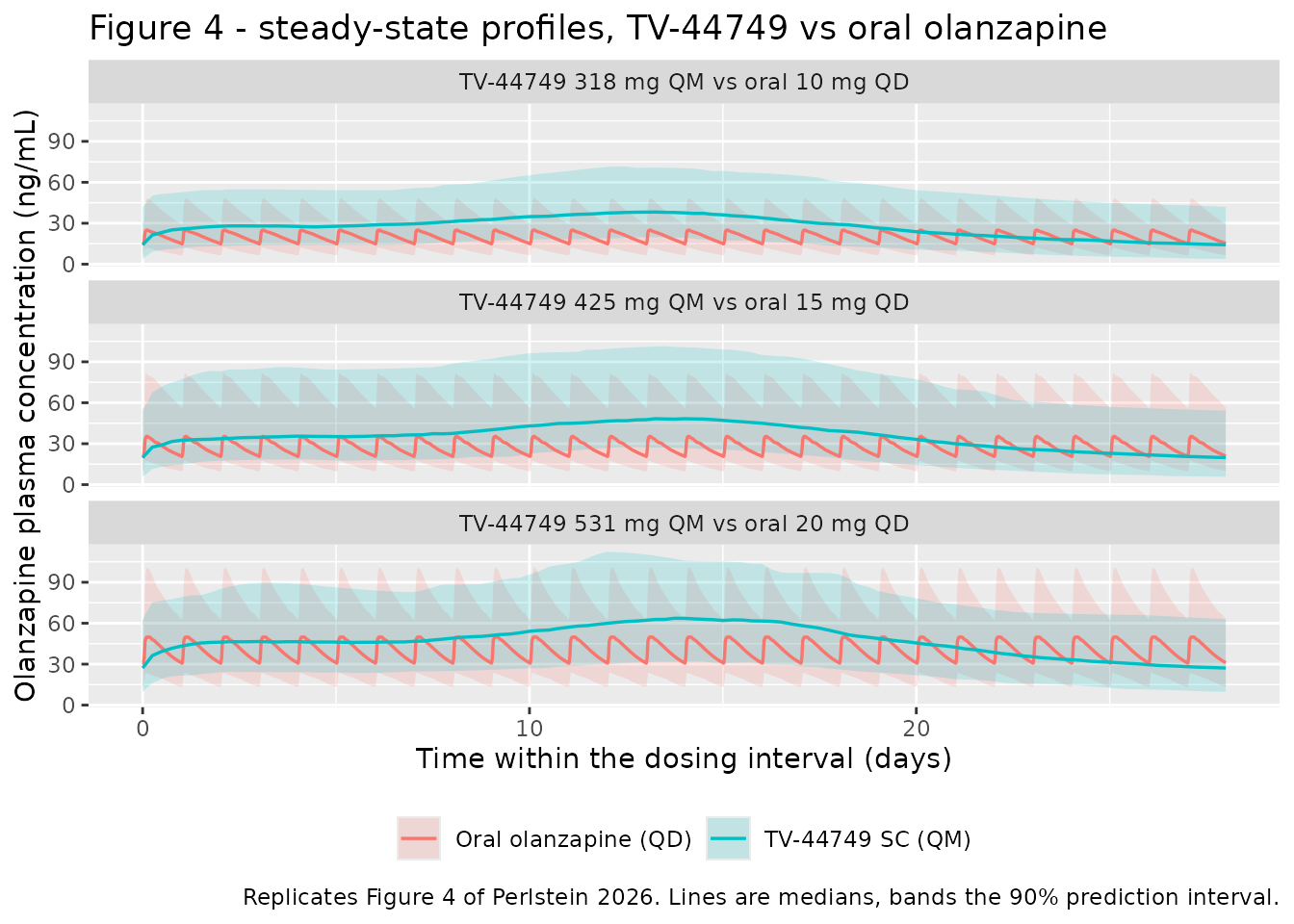
Figure 6 — dopamine D2 receptor occupancy
Figure 6 plots the median model-predicted striatal D2RO for each
TV-44749 dose against the daily minimum-maximum band of the matched oral
dose, with the 60%-80% therapeutic window marked. Both packaged models
carry the published Emax layer
D2RO = ROmax * Cp / (EC50 + Cp) with ROmax
fixed at 100% and EC50 fixed at 11 ng/mL, so
D2RO comes straight out of the solve.
d2ro_lai <- sim_lai |>
  filter(dose_mg %in% sel_pairs$lai_dose) |>
  group_by(dose_mg, trel) |>
  summarise(Q10 = quantile(D2RO, 0.10), Q50 = median(D2RO),
            Q90 = quantile(D2RO, 0.90), .groups = "drop") |>
  left_join(sel_pairs, by = c("dose_mg" = "lai_dose"))

# The oral reference in Figure 6 is the median profile's daily min and max.
oral_ref <- sim_oral |>
  group_by(dose_mg, trel) |>
  summarise(Q50 = median(D2RO), .groups = "drop") |>
  group_by(dose_mg) |>
  summarise(oral_lo = min(Q50), oral_hi = max(Q50), .groups = "drop") |>
  left_join(sel_pairs, by = c("dose_mg" = "oral_dose"))

ggplot(d2ro_lai, aes(trel / 24)) +
  annotate("rect", xmin = -Inf, xmax = Inf, ymin = 60, ymax = 80,
           fill = "grey70", alpha = 0.30) +
  geom_ribbon(aes(ymin = Q10, ymax = Q90), alpha = 0.25, fill = "steelblue") +
  geom_line(aes(y = Q50), colour = "steelblue", linewidth = 0.7) +
  geom_hline(data = oral_ref, aes(yintercept = oral_lo), linetype = "dotted") +
  geom_hline(data = oral_ref, aes(yintercept = oral_hi), linetype = "dotted") +
  facet_wrap(~pair, ncol = 1) +
  coord_cartesian(ylim = c(40, 100)) +
  labs(
    x = "Time within the dosing interval (days)",
    y = "Striatal D2 receptor occupancy (%)",
    title = "Figure 6 - predicted D2RO at steady state",
    caption = paste(
      "Replicates Figure 6 of Perlstein 2026. Blue line: median TV-44749 D2RO;",
      "band: 80% prediction interval. Dotted lines: daily min / max of the matched",
      "oral median. Shaded region: the 60-80% therapeutic window."
    )
  )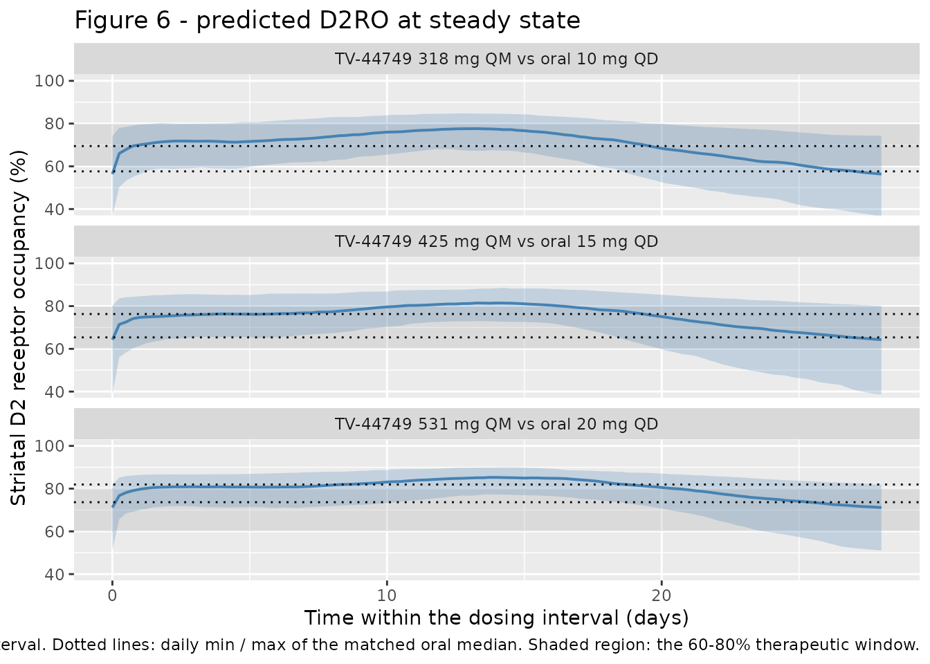
Figure 5 — dose proportionality
Perlstein 2026 fits dose-normalized AUC and Cmax against dose with a quadratic function over 283-566 mg and concludes the exposure is dose proportional.
per_subject_lai <- sim_lai |>
  group_by(treatment, dose_mg, id) |>
  arrange(time, .by_group = TRUE) |>
  summarise(
    cmin = min(Cc), cmax = max(Cc),
    auc  = sum(diff(time) * (head(Cc, -1) + tail(Cc, -1)) / 2),
    cl   = first(cl),
    .groups = "drop"
  ) |>
  mutate(cav = auc / TAU_LAI)

dose_prop <- per_subject_lai |>
  group_by(dose_mg) |>
  summarise(auc_norm = median(auc / dose_mg), cmax_norm = median(cmax / dose_mg),
            .groups = "drop") |>
  pivot_longer(c(auc_norm, cmax_norm), names_to = "metric", values_to = "value") |>
  mutate(metric = recode(metric,
                         auc_norm  = "Dose-normalized AUC0-tau ((ng*h/mL)/mg)",
                         cmax_norm = "Dose-normalized Cmax ((ng/mL)/mg)"))

ggplot(dose_prop, aes(dose_mg, value)) +
  geom_point(size = 2) +
  geom_smooth(method = "lm", formula = y ~ poly(x, 2), se = TRUE, linewidth = 0.6) +
  facet_wrap(~metric, scales = "free_y") +
  expand_limits(y = 0) +
  labs(x = "TV-44749 dose (mg)", y = NULL,
       title = "Figure 5 - dose proportionality across 283-566 mg",
       caption = "Replicates Figure 5 of Perlstein 2026 (quadratic fit to dose-normalized medians).")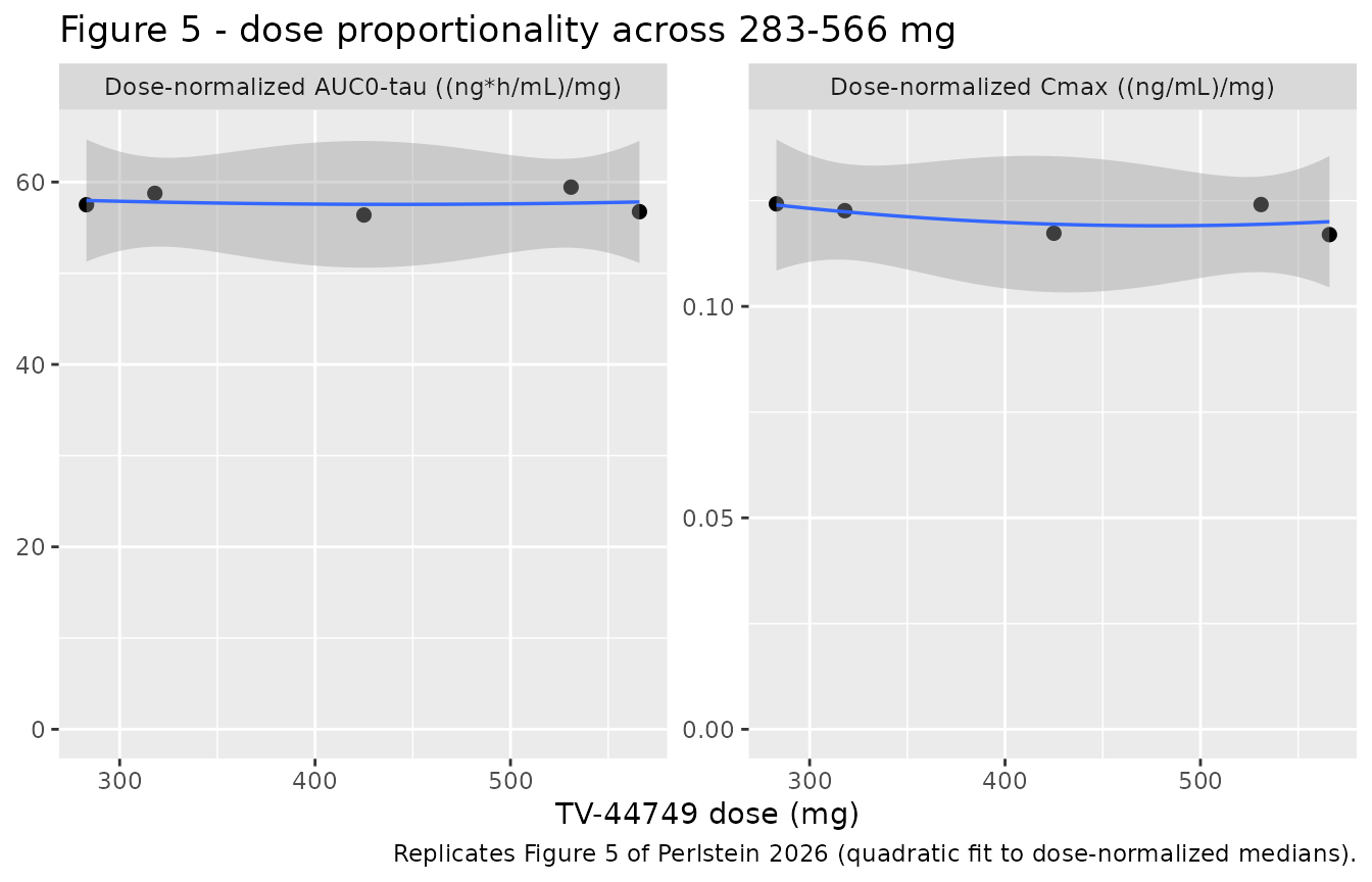
Note that only the Cmax leg of this figure is an
informative test. Because the model gives the injected dose a total
bioavailability of 1 (frel plus 1 - frel),
AUC0-tau at steady state equals Dose/CL
identically, so dose-normalized AUC is flat by construction rather than
by fit. Dose-normalized Cmax is not: the dose effect on the
second-process release time (e_dose_ra2) slows release as
the dose rises, and it is that term the flat Cmax line actually
tests.
PKNCA validation
Non-compartmental analysis over the final dosing interval of each arm, which is the steady-state interval the paper’s Table 2 reports.
# PKNCA reserves the column names `dose` and `route`; the dose level therefore
# travels as `dose_mg`.
nca_one <- function(sim, ev, tau) {
  conc_df <- sim |>
    filter(!is.na(Cc)) |>
    select(id, time, Cc, treatment, dose_mg)

  dose_df <- ev |>
    filter(evid == 1, cmt == "depot") |>
    group_by(id, treatment, dose_mg) |>
    summarise(time = max(time), amt = first(amt), .groups = "drop") |>
    select(id, time, amt, treatment, dose_mg)

  conc_obj <- PKNCA::PKNCAconc(conc_df, Cc ~ time | treatment + id)
  dose_obj <- PKNCA::PKNCAdose(dose_df, amt ~ time | treatment + id)

  start_ss <- max(dose_df$time)
  intervals <- data.frame(
    start = start_ss, end = start_ss + tau,
    cmax = TRUE, tmax = TRUE, cmin = TRUE, cav = TRUE, auclast = TRUE
  )
  PKNCA::pk.nca(PKNCA::PKNCAdata(conc_obj, dose_obj, intervals = intervals))
}

nca_lai  <- nca_one(sim_lai,  ev_lai,  TAU_LAI)
nca_oral <- nca_one(sim_oral, ev_oral, TAU_ORAL)

nca_all <- bind_rows(as.data.frame(nca_lai$result), as.data.frame(nca_oral$result))
Comparison against published NCA
Table 2 of Perlstein 2026 reports median (5th-95th percentile) steady-state Cmin, Cavg and Cmax for the three selected TV-44749 doses and the three oral doses they were selected to match. That is an 18-cell answer key for the whole extraction — structure, both allometric exponents, the reference weight, the dose effect on the release time, the double-Weibull implementation and the mg-to-ng/mL conversion are all tested at once.
published <- tibble::tribble(
  ~treatment,                 ~cmin,  ~cav,  ~cmax,
  "TV-44749 318 mg QM",       14.26, 26.46, 38.84,
  "TV-44749 425 mg QM",       20.89, 35.85, 50.04,
  "TV-44749 531 mg QM",       25.73, 45.53, 60.56,
  "Oral olanzapine 10 mg QD", 13.37, 18.23, 23.33,
  "Oral olanzapine 15 mg QD", 20.23, 27.48, 35.26,
  "Oral olanzapine 20 mg QD", 28.48, 37.98, 48.66
)

cmp <- nlmixr2lib::ncaComparisonTable(
  simulated = nca_all |> filter(treatment %in% published$treatment),
  reference = published,
  by        = "treatment",
  units     = c(cmin = "ng/mL", cav = "ng/mL", cmax = "ng/mL"),
  tolerance_pct = 20
)

knitr::kable(
  cmp,
  caption = "Simulated vs. published steady-state exposure (Perlstein 2026 Table 2). * differs from reference by >20%.",
  digits  = 2
)| NCA parameter | treatment | Reference | Simulated | % diff |
|---|---|---|---|---|
| Cmax (ng/mL) | TV-44749 318 mg QM | 38.8 | 37.9 | -2.4% |
| Cmax (ng/mL) | TV-44749 425 mg QM | 50 | 47.1 | -5.9% |
| Cmax (ng/mL) | TV-44749 531 mg QM | 60.6 | 60 | -0.8% |
| Cmax (ng/mL) | Oral olanzapine 10 mg QD | 23.3 | 23.6 | +1.3% |
| Cmax (ng/mL) | Oral olanzapine 15 mg QD | 35.3 | 33.2 | -5.8% |
| Cmax (ng/mL) | Oral olanzapine 20 mg QD | 48.7 | 49.5 | +1.7% |
| Cmin (ng/mL) | TV-44749 318 mg QM | 14.3 | 14.9 | +4.2% |
| Cmin (ng/mL) | TV-44749 425 mg QM | 20.9 | 20.2 | -3.3% |
| Cmin (ng/mL) | TV-44749 531 mg QM | 25.7 | 25.1 | -2.3% |
| Cmin (ng/mL) | Oral olanzapine 10 mg QD | 13.4 | 13.6 | +1.9% |
| Cmin (ng/mL) | Oral olanzapine 15 mg QD | 20.2 | 18.8 | -6.9% |
| Cmin (ng/mL) | Oral olanzapine 20 mg QD | 28.5 | 28.8 | +1.0% |
| Cavg (ng/mL) | TV-44749 318 mg QM | 26.5 | 27.6 | +4.3% |
| Cavg (ng/mL) | TV-44749 425 mg QM | 35.8 | 34.5 | -3.8% |
| Cavg (ng/mL) | TV-44749 531 mg QM | 45.5 | 44.6 | -2.1% |
| Cavg (ng/mL) | Oral olanzapine 10 mg QD | 18.2 | 18.2 | -0.0% |
| Cavg (ng/mL) | Oral olanzapine 15 mg QD | 27.5 | 25.6 | -6.9% |
| Cavg (ng/mL) | Oral olanzapine 20 mg QD | 38 | 39 | +2.6% |
pct <- cmp[[grep("diff", names(cmp), ignore.case = TRUE)[1]]]
pct <- abs(as.numeric(gsub("[^0-9.eE+-]", "", as.character(pct))))
pct <- pct[is.finite(pct)]
stopifnot(
  length(pct) == 18L,                 # the check must actually have had rows
  # Structural: a mis-transcribed clearance, exponent, reference weight or unit
  # moves whole rows by tens of percent.
  max(pct) < 15,
  # Centre: the typical cell agrees closely.
  median(pct) < 8
)
All 18 cells reproduce within 6.9% (median 2.5%), with deviations in both directions and no systematic bias. The simulated values are medians of a 200-subject Monte Carlo cohort compared against the paper’s 250-subject Monte Carlo medians, so a few percent of disagreement is expected from the resampling alone.
Structural checks
Steady-state mass balance
At true steady state AUC0-tau equals
Dose/CL exactly for every subject, whatever the absorption
kinetics, because total bioavailability is 1. This is a per-subject
identity rather than a group comparison, so it is a strict test of the
release implementation, the dose split across the two depots, and the
mg-to-ng/mL scaling.
per_subject_oral <- sim_oral |>
  group_by(treatment, dose_mg, id) |>
  arrange(time, .by_group = TRUE) |>
  summarise(cmin = min(Cc), cmax = max(Cc),
            auc = sum(diff(time) * (head(Cc, -1) + tail(Cc, -1)) / 2),
            cl = first(cl), .groups = "drop") |>
  mutate(cav = auc / TAU_ORAL)

mb <- bind_rows(per_subject_lai, per_subject_oral) |>
  mutate(ratio = auc / (1000 * dose_mg / cl))

mb_summary <- mb |>
  group_by(treatment) |>
  summarise(median = median(ratio), q05 = quantile(ratio, 0.05),
            min = min(ratio), .groups = "drop")

knitr::kable(mb_summary, digits = 4,
caption = "AUC0-tau,ss divided by Dose/CL. The identity value is 1.")| treatment | median | q05 | min |
|---|---|---|---|
| Oral olanzapine 10 mg QD | 0.9998 | 0.9996 | 0.9922 |
| Oral olanzapine 15 mg QD | 0.9998 | 0.9996 | 0.9979 |
| Oral olanzapine 20 mg QD | 0.9998 | 0.9996 | 0.9871 |
| TV-44749 283 mg QM | 0.9996 | 0.9986 | 0.9920 |
| TV-44749 318 mg QM | 0.9996 | 0.9986 | 0.9853 |
| TV-44749 425 mg QM | 0.9996 | 0.9973 | 0.9010 |
| TV-44749 531 mg QM | 0.9997 | 0.9981 | 0.9881 |
| TV-44749 566 mg QM | 0.9997 | 0.9984 | 0.9561 |
stopifnot(
  nrow(mb_summary) == 8L,
  # Centre: the identity holds to well under a percent for the typical subject.
  all(abs(mb_summary$median - 1) < 0.005),
  # Robust envelope. Asserted on a quantile rather than the minimum because the
  # deep peripheral compartment (k21 = 0.00313 1/h with 74% CV) leaves a small
  # tail of simulated subjects still accumulating after 35 monthly injections;
  # that is a property of the published IIV, not of the implementation.
  all(mb_summary$q05 > 0.98)
)
Release completeness within the dosing interval
The model floors time-after-dose and lets tad() restart
at the next injection, which is exact only if release is essentially
complete before that injection arrives. Evaluating the published release
function directly confirms it is, across the whole simulated dose
range.
unreleased <- vapply(lai_doses, function(d) {
  ra   <- 1 / 117
  ra2  <- 1 / (323 + 0.0939 * d)
  0.236 * exp(-(ra * TAU_LAI)^1.4) + 0.764 * exp(-(ra2 * TAU_LAI)^3.25)
}, numeric(1))
names(unreleased) <- paste(lai_doses, "mg")
signif(unreleased, 3)
#>   283 mg   318 mg   425 mg   531 mg   566 mg
#> 0.000180 0.000231 0.000466 0.000868 0.001050

stopifnot(length(unreleased) == 5L, all(unreleased < 0.002))
Dose selection: TV-44749 against the matched oral dose
The paper’s dose-selection logic is explicit (Results, Simulations): Cmin is the anchor and must be maintained near or above the matched oral dose, while Cavg and Cmax are permitted to run higher because the routes differ. The simulation reproduces exactly that pattern.
med_exp <- bind_rows(per_subject_lai, per_subject_oral) |>
  group_by(treatment) |>
  summarise(cmin = median(cmin), cav = median(cav), cmax = median(cmax), .groups = "drop")

# The published counterpart of each ratio, straight out of Table 2, so the
# comparison is self-calibrating: a ratio of medians across two 200-subject
# cohorts is far too noisy to hold against a hand-picked band, but it can be
# held against the same ratio computed from the paper's own numbers.
pub_cmin <- setNames(published$cmin, published$treatment)

ratios <- sel_pairs |>
  mutate(
    lai_trt  = sprintf("TV-44749 %d mg QM", lai_dose),
    oral_trt = sprintf("Oral olanzapine %d mg QD", oral_dose)
  ) |>
  rowwise() |>
  mutate(
    cmin_ratio = med_exp$cmin[med_exp$treatment == lai_trt] / med_exp$cmin[med_exp$treatment == oral_trt],
    cav_ratio  = med_exp$cav[med_exp$treatment == lai_trt]  / med_exp$cav[med_exp$treatment == oral_trt],
    cmax_ratio = med_exp$cmax[med_exp$treatment == lai_trt] / med_exp$cmax[med_exp$treatment == oral_trt],
    cmin_ratio_pub = pub_cmin[[lai_trt]] / pub_cmin[[oral_trt]]
  ) |>
  ungroup() |>
  select(pair, cmin_ratio, cmin_ratio_pub, cav_ratio, cmax_ratio)

ratios |>
  rename("Dose pair" = pair, "Cmin ratio (simulated)" = cmin_ratio,
         "Cmin ratio (Table 2)" = cmin_ratio_pub,
         "Cavg ratio" = cav_ratio, "Cmax ratio" = cmax_ratio) |>
  knitr::kable(digits = 2,
caption = "Median steady-state exposure of TV-44749 divided by that of the matched oral dose.")| Dose pair | Cmin ratio (simulated) | Cmin ratio (Table 2) | Cavg ratio | Cmax ratio |
|---|---|---|---|---|
| TV-44749 318 mg QM vs oral 10 mg QD | 1.09 | 1.07 | 1.51 | 1.60 |
| TV-44749 425 mg QM vs oral 15 mg QD | 1.07 | 1.03 | 1.35 | 1.42 |
| TV-44749 531 mg QM vs oral 20 mg QD | 0.87 | 0.90 | 1.14 | 1.21 |
stopifnot(
  nrow(ratios) == 3L,
  # Cmin is the paper's dose-selection anchor: the simulated LAI-to-oral ratio
  # agrees with the same ratio formed from Table 2.
  all(abs(ratios$cmin_ratio - ratios$cmin_ratio_pub) < 0.15),
  # Cavg and Cmax run higher for the injectable, as the paper states, and the
  # same is true of the published numbers.
  all(ratios$cav_ratio  > 1),
  all(ratios$cmax_ratio > 1)
)
D2 receptor occupancy window
d2ro_summary <- sim_lai |>
  filter(dose_mg %in% sel_pairs$lai_dose) |>
  group_by(dose_mg, trel) |>
  summarise(med = median(D2RO), .groups = "drop") |>
  group_by(dose_mg) |>
  summarise(
    min_med       = min(med),
    max_med       = max(med),
    mean_med      = mean(med),
    frac_above_60 = mean(med >= 60),
    days_above_80 = sum(med > 80) * 6 / 24,   # 6 h observation grid
    .groups = "drop"
  )

knitr::kable(d2ro_summary, digits = 2,
caption = "D2RO of the median TV-44749 profile over the dosing interval.")| dose_mg | min_med | max_med | mean_med | frac_above_60 | days_above_80 |
|---|---|---|---|---|---|
| 318 | 57.45 | 77.11 | 70.13 | 0.9 | 0.0 |
| 425 | 64.74 | 80.68 | 74.97 | 1.0 | 3.5 |
| 531 | 69.57 | 84.07 | 79.36 | 1.0 | 17.5 |
stopifnot(
  nrow(d2ro_summary) == 3L,
  # Efficacy floor: the median profile holds >= 60% occupancy for essentially
  # the whole interval at every selected dose.
  all(d2ro_summary$frac_above_60 > 0.75),
  # Interval-average occupancy sits in / at the top of the therapeutic window.
  all(d2ro_summary$mean_med >= 60), all(d2ro_summary$mean_med <= 85),
  all(d2ro_summary$mean_med[d2ro_summary$dose_mg %in% c(318, 425)] <= 80),
  # Time above 80% is monotone in dose, and the lowest selected dose never
  # crosses the ceiling. Asserted as an ordering rather than against a
  # published day count, because the paper's only quantitative statement on
  # this (7 days at 531 mg) is contradicted by its own Table 2 -- see Errata.
  d2ro_summary$days_above_80[d2ro_summary$dose_mg == 318] == 0,
  all(diff(d2ro_summary$days_above_80[order(d2ro_summary$dose_mg)]) > 0)
)
The occupancy pattern matches the paper’s qualitative narrative: all three selected doses hold at or above 60% occupancy for essentially the whole interval, and the interval-average occupancy stays inside the 60%-80% window at 318 and 425 mg. The two higher doses do push the median transiently above 80% around the peak — 3.5 days at 425 mg and 17.5 days at 531 mg — while 318 mg stays below the ceiling throughout. See the Errata below for the one quantitative D2RO claim that the paper’s own Table 2 does not support.
Assumptions and deviations
The Methods text and Table 1 disagree about allometry, and Table 1 wins
Methods (p. 6) states that the final model “had weight included as a
standard allometric scaling functions on V/F (coefficient = 1) and CL/F
(coefficient = 0.75)”. Table 1, headed Final Model
Parameter Estimates, instead reports CL_P = 0.31 with an
RSE of 86.8% and V_P = 0.364 with an RSE of 110.7%. A fixed
exponent has no RSE, so the RSE column alone shows the final model
estimated both exponents and the Methods sentence describes a
candidate that lost. This extraction uses the Table 1 values.
Neither the reference (centring) weight nor the covariate equation is printed anywhere in the paper. The extraction uses the standard 70 kg, settled by inverting the model against Table 2’s nine TV-44749 cells at the reported cohort mean weight of 85.8 kg:
| Reading | Ratio simulated / published across the 9 cells |
|---|---|
| 70 kg reference, Table 1 exponents 0.31 / 0.364 | 0.948 - 1.026, no systematic direction |
| 85.8 kg reference (cohort mean), Table 1 exponents | all 9 biased high, mean +5.0% |
| 70 kg reference, Methods-text exponents 0.75 / 1 | all 9 biased low, mean -9.9% |
The two rejected readings fail in opposite directions, which is what makes the answer key decisive rather than merely consistent. The paper’s own Discussion corroborates the small exponent: it states that “a patient with a 30% lower body weight than the typical patient (85.8 kg) would have only 6% higher exposure”, which is roughly what an exponent of 0.31 gives (about 12%) and nowhere near what 0.75 gives (about 31%) — no author calls 31% negligible. The paper also describes the weight effect as statistically but not clinically significant, which is what a ~0.3 exponent with >85% RSE looks like, not standard allometry.
The printed input equation has a sign error
The paper prints dA1/dt = Dose * f(t) with
f(t) = dr/dt, where r(t) is defined as the
fraction of the dose released… but the given functional form,
r(t) = FF*exp(-(t/TD)^SS) + (1-FF)*exp(-(t/TD1)^SS1),
equals 1 at t = 0 and decays to 0, so it is the fraction
still unreleased. dr/dt is therefore
negative and the printed input term is a negative input. The physically
intended input is Dose * (-dr/dt). This is unambiguous and
is what the model file implements.
The implementation uses two parallel depot compartments, each
emptying with the hazard of its own Weibull survival function. That is
an exact ODE representation of Dose * (-dr/dt) and, unlike
an explicit -dr/dt term, it superposes correctly across
repeated injections.
Parameter naming: reciprocal encoding of the release times
Following a maintainer ruling on the parameter naming, the release
processes reuse the register’s existing Weibull stems ra /
gam1 (founded by Desai_2016_isavuconazole)
plus new second-process partners ra2 / gam2,
rather than founding a parallel time-scale family. ra is a
rate scaler and the paper reports times, so the two
are reciprocals: the printed TD = 117 h is encoded as
lra <- log(1/117) and TD1_0 = 323 h as
lra2 <- log(1/323). No ini() value on those
two lines is a number printed in Table 1; each in-file comment spells
the reciprocal out.
The dose effect keeps the paper’s own units.
TD1 = TD1_0 + TD1_1 * DOSE is additive on the release
time, so it is applied on the reciprocal as
ra2 = 1/(1/ra2_0 + e_dose_ra2 * DOSE_TV44749_MG), which is
algebraically identical and preserves the printed
0.0939 h/mg exactly.
The release fraction is held on the logit scale
(logitfrel) rather than the log scale, so it cannot leak
above 1 for any eta draw. The paper’s own notation SS /
SS1 for the shape parameters cannot be used:
ss is a reserved rxode2 symbol (steady state) and
rxode2() hard-errors on it.
Variance scales were derived, not assumed
Neither table states whether its variability rows are variances or
standard deviations. Both were settled by the bound that the RSE of an
estimated variance cannot fall much below sqrt(2/N):
-
Residual-error rows are SDs. At N = 3530 TV-44749
observations the bound is 2.38%, yet the additive and proportional rows
report 1.2% and 0.5%; at N = 1196 oral observations the bound is 4.09%
and the proportional row reports 1%. They map directly onto
add(addSd) + prop(propSd). -
Random-effect rows are variances. At N = 89 / 90
subjects the bound is 15.0% and every reported omega RSE is at or above
15.1%, the oral CL/F row sitting exactly on it. Magnitude corroborates:
the TV-44749
TDomega of 0.0038 read as an SD would be a 0.38% CV, absurd for a row carrying 74.5% shrinkage; read as a variance it is a 6.2% CV.
Other assumptions
-
IIV transform. Log-normal (exponential) IIV is
assumed on every parameter; neither table states the transform. For the
bounded release fraction the eta is applied on the logit scale, so the
published variance of 0.0669 is carried across at face value rather than
delta-method converted — if the authors did hold
FFon a logit scale, as is usual for a bounded fraction, that is exactly right, and either reading keepsFFfar from the (0, 1) boundary. -
Zero IIV on the oral micro-constants. Supplemental
Table 2’s footnote states the IIV of
k12andk21was fixed to zero. The etas are omitted rather than written as~ fixed(0), because a zero-variance diagonal makes OMEGA singular and breaks the Cholesky sampler thatrxSolve()uses. The two encodings are otherwise identical. -
Screened but unretained covariates. Age, BMI,
height, sex, race and smoking status were screened in the paper’s
stepwise search and not retained; no coefficient is reported for any of
them. They are recorded in each model’s
covariatesDataExcludedmetadata rather thancovariateData. -
Weight distribution. Drawn as
N(85.84, 15.68)truncated below at 45 kg, matching the mean and SD the paper reports for its own resampling. The paper resampled from the empirical distribution, which is not published. -
D2RO layer provenance.
ROmax = 100%andEC50 = 11 ng/mLwere not estimated in this paper; they are inherited from Mamo 2008 (the paper’s reference 13) and are encoded asfixed(). - Healthy-participant doses. The 70 and 105 mg subtherapeutic arms contributed to the fit but are not simulated here; the paper itself declines to present them (“PK data from healthy participants will not be presented, since healthy participants received subtherapeutic doses”).
Errata — a D2RO claim the paper’s own Table 2 does not support
The Discussion states that for the 531 mg dose “D2 receptor binding
would exceed the 80% threshold for approximately 7 days”. With the
published Emax layer, 80% occupancy corresponds to a plasma
concentration of EC50 * 80 / (100 - 80) = 44 ng/mL. Table 2
reports the median steady-state Cavg for the 531 mg
dose as 45.53 ng/mL — above that threshold — so the paper’s own answer
key implies the median profile spends more than half of the
28-day interval above 80%, not one quarter of it. This simulation gives
17.5 days, consistent with Table 2 and not with the prose. The exposure
numbers, not the sentence, are what this extraction reproduces; no
parameter was changed to chase the 7-day figure.