Ciclosporin (Press 2010)
Source:vignettes/articles/Press_2010_ciclosporin.Rmd
Press_2010_ciclosporin.RmdModel and source
- Citation: Press RR, Ploeger BA, den Hartigh J, van der Straaten T, van Pelt H, Danhof M, de Fijter H, Guchelaar HJ. Explaining variability in ciclosporin exposure in adult kidney transplant recipients. Eur J Clin Pharmacol. 2010;66(6):579-590. doi:10.1007/s00228-010-0810-9.
- Description: Two-compartment population pharmacokinetic model for oral ciclosporin A (Neoral) in adult kidney transplant recipients (Press 2010). Delayed absorption is described by one transit compartment with the first-order transit rate constant set equal to the absorption rate constant ka (chain: depot -> transit1 -> central at common rate ka; mean absorption time = (n+1)/ka with n = 1 transit compartment). Oral bioavailability is FIXED at 0.5 (Methods ‘Structural model’). Apparent clearance CL and apparent central volume of distribution Vc are allometrically scaled to body weight at a 76 kg median reference with theory-based exponents 0.75 on CL and 1.0 on Vc; the peripheral volume Vp and intercompartmental clearance Q are not weight-scaled. Concomitant high-dose oral prednisolone (PRED_DOSE >= 20 mg/day) is associated with a 55% reduction in the absorption rate constant and a 22% reduction in bioavailability (binary threshold-form covariate). Inter-occasion variability on bioavailability is encoded here as IIV on lfdepot because the source does not specify a per-subject occasion count for downstream simulation (see vignette Assumptions and deviations).
- Article: https://doi.org/10.1007/s00228-010-0810-9
Population
Press 2010 followed n = 33 de novo adult kidney transplant recipients for one year after transplantation, recruited at the Leiden University Medical Center (Netherlands). Patients received quadruple immunosuppression: basiliximab induction (day 0 and day 4), fixed-dose mycophenolate mofetil (1,000 mg twice daily), tapering prednisolone (50 mg twice daily on day 0, tapered to 10 mg once daily by day 22), and ciclosporin A (Neoral) 8 mg/kg/day, randomized to once-daily (n = 17) or twice-daily (n = 16) administration. Therapeutic drug monitoring (TDM) targeted AUC0-24h 10,800 microgh/L (once daily) or AUC0-12h 5,400 microgh/L (twice daily) in the first 6 weeks post-transplant, then 6,500 microgh/L or 3,250 microgh/L respectively thereafter (Table 1, Methods page 580). Recipient demographics (combined arms): mean age 46 years (range 18 - 70), 79% male, 79% Caucasian, body weight 49 - 140 kg (median 76 kg).
Sampling was dense: at weeks 2, 6, 12, 26, and 52 each patient was sampled at t = 0, 1, 2, 3, 4, 6 and 24 h; routine TDM (t = 0, 2, 3 h) was added at weeks 4, 8, 10, 17, 21 and 39. Twenty-two of the 33 patients contributed eleven sampling occasions across the year. Whole- blood ciclosporin was assayed by FPIA (Abbott TDx) with inter-day CV 10.4% / 7.8% / 7.5% at 70 / 300 / 600 microg/L (Methods page 581).
The same information is available programmatically via
rxode2::rxode(readModelDb("Press_2010_ciclosporin"))$population.
Source trace
The per-parameter origin is recorded as a trailing in-file comment
next to each ini() entry in
inst/modeldb/specificDrugs/Press_2010_ciclosporin.R. The
table below collects them in one place for review.
| Equation / parameter | Value | Source location (Press 2010) |
|---|---|---|
| Two-compartment disposition with first-order elimination | n/a | Results ‘CsA pharmacokinetic model’, Fig. 1 |
| One transit compartment with rate = ka (depot -> transit1 -> central) | n/a | Results ‘CsA pharmacokinetic model’; Table 4 ‘Number of transit compartments = 1’ |
| Mean transit time = (n + 1)/ka = 2/ka = 1 h at ka = 2 | n/a | Results: “transit time can be calculated with 1/ka*(n+1)” |
lka (ka) |
log(2.0) -> 2.0 1/h | Table 4 ‘Absorption rate constant’ mean value |
lcl (CL at WT 76 kg) |
log(15) -> 15 L/h | Table 4 ‘CsA clearance’ mean value; Results: CL = 15 * (WT/76)^0.75 |
lvc (Vc at WT 76 kg) |
log(56) -> 56 L | Table 4 ‘Central volume of distribution’ mean value |
lvp (Vp) |
log(125) -> 125 L | Table 4 ‘Peripheral volume of distribution’ mean value |
lq (Q) |
log(14) -> 14 L/h | Table 4 ‘Intercompartmental clearance’ mean value |
lfdepot (F, FIXED) |
log(0.5) -> 0.5 | Methods ‘Structural model’: “fixed at 50%, as previously described” |
allo_cl (WT exponent on CL, FIXED) |
0.75 | Results: “typically with a value of 0.75 for clearance” |
allo_vc (WT exponent on Vc, FIXED) |
1.0 | Results: “and 1 for volume of distribution” |
e_pred_dose_high_ka (ka effect when PRED_DOSE >= 20
mg/day) |
-0.55 | Table 4 footnote b; delta-OFV = +233 on deletion |
e_pred_dose_high_f (F effect when PRED_DOSE >= 20
mg/day) |
-0.22 | Table 4 footnote b; delta-OFV = +51 on deletion |
etalka IIV variance |
0.09 (CV 30%) | Table 4 ‘IIV absorption rate’ |
etalcl IIV variance |
0.03 (CV 17%) | Table 4 ‘IIV clearance’ |
etalvc IIV variance |
0.12 (CV 35%) | Table 4 ‘IIV central volume of distribution’ |
etalfdepot (IOV on F encoded as IIV) variance |
0.02 (CV 14%) | Table 4 ‘IOV bioavailability’ |
propSd (proportional residual SD) |
sqrt(0.07) ~ 0.265 | Methods ‘Random effects’: log(Cij) = log(Cpredij) + eps; Table 4 sigma^2 = 0.07 |
Virtual cohort
The virtual cohort uses two strata corresponding to the post-transplant prednisolone taper (Methods page 580):
- Early post-transplant (HIGH prednisolone, days 0-21): PRED_DOSE = 100 mg/day on day 0 tapering to 10 mg/day by day 22; the HIGH-dose covariate (>= 20 mg/day) flips OFF around day 14. For the steady-state simulation we hold PRED_DOSE = 30 mg/day (above the 20 mg/day threshold), representative of weeks 1 - 2 post-transplant.
- Stable maintenance (LOW prednisolone, day 22+): PRED_DOSE = 10 mg/day (below the threshold), representative of weeks 4 - 52.
Both cohorts receive 4 mg/kg of ciclosporin A every 12 h (the starting twice-daily regimen, before TDM dose adjustment), reaching steady state by the end of day 5.
set.seed(2010)

# Helper: build one cohort as a self-contained event table.
make_cohort <- function(n, dose_mg_per_kg, pred_dose_mg_day, treatment,
                        id_offset = 0L) {
  # Approximate the Press 2010 weight distribution: log-normal centred on
  # the cohort median (76 kg) with a CV that reproduces a 49-140 kg span
  # over the central 95% (CV ~ 0.22 on the log scale).
  weights <- exp(rnorm(n, mean = log(76), sd = 0.22))

  dose_times <- seq(0, by = 12, length.out = 10)        # 5 days BID
  ss_offset  <- 96                                       # start of 9th interval
  obs_grid   <- ss_offset + c(0, 0.5, 1, 1.5, 2, 2.5, 3, 4, 5, 6, 8, 10, 12)

  cohort <- tibble::tibble(
    id        = id_offset + seq_len(n),
    WT        = weights,
    PRED_DOSE = pred_dose_mg_day,
    treatment = treatment
  )

  dplyr::bind_rows(
    cohort |>
      tidyr::expand_grid(time = dose_times) |>
      dplyr::mutate(
        amt  = dose_mg_per_kg * WT,
        evid = 1L,
        cmt  = "depot"
      ),
    cohort |>
      tidyr::expand_grid(time = obs_grid) |>
      dplyr::mutate(
        amt  = 0,
        evid = 0L,
        cmt  = "central"
      )
  ) |>
    dplyr::arrange(id, time, dplyr::desc(evid))
}

events <- dplyr::bind_rows(
  make_cohort(n = 100, dose_mg_per_kg = 4, pred_dose_mg_day = 30,
              treatment = "Early (HIGH PRED >=20)", id_offset =   0L),
  make_cohort(n = 100, dose_mg_per_kg = 4, pred_dose_mg_day = 10,
              treatment = "Maintenance (LOW PRED <20)", id_offset = 100L)
)

stopifnot(!anyDuplicated(unique(events[, c("id", "time", "evid")])))
Simulation
mod <- readModelDb("Press_2010_ciclosporin")

sim <- rxode2::rxSolve(
  mod,
  events = events,
  keep   = c("treatment", "WT", "PRED_DOSE")
) |>
  as.data.frame()

mod_typ <- rxode2::zeroRe(mod)
sim_typ <- rxode2::rxSolve(
  mod_typ,
  events = events,
  keep   = c("treatment", "WT", "PRED_DOSE")
) |>
  as.data.frame()
#> ℹ omega/sigma items treated as zero: 'etalka', 'etalcl', 'etalvc', 'etalfdepot'
#> Warning: multi-subject simulation without without 'omega'
Replicate Figure 2: steady-state visual predictive check
Press 2010 Figure 2 displays the model VPC against the observed ciclosporin A concentrations across the population. The packaged model should reproduce the characteristic absorption + biphasic disposition shape, with the HIGH-prednisolone stratum showing both slower absorption (55% lower ka -> later peak) and lower exposure (22% lower F).
ss_offset <- 96   # start of last full dosing interval used for VPC

vpc <- sim |>
  dplyr::filter(!is.na(Cc), time >= ss_offset) |>
  dplyr::mutate(tad = time - ss_offset) |>
  dplyr::group_by(treatment, tad) |>
  dplyr::summarise(
    Q10 = quantile(Cc, 0.10, na.rm = TRUE),
    Q50 = quantile(Cc, 0.50, na.rm = TRUE),
    Q90 = quantile(Cc, 0.90, na.rm = TRUE),
    .groups = "drop"
  )

ggplot(vpc, aes(x = tad, y = Q50, colour = treatment, fill = treatment)) +
  geom_ribbon(aes(ymin = Q10, ymax = Q90), alpha = 0.20, colour = NA) +
  geom_line(linewidth = 0.7) +
  scale_y_log10() +
  labs(
    x = "Time after dose (h)",
    y = "Whole-blood ciclosporin (microg/L, log scale)",
    title = "Steady-state VPC, 4 mg/kg BID",
    caption = paste(
      "Median + 80% prediction interval, n = 100 virtual subjects per",
      "stratum. Replicates the layout of Press 2010 Figure 2 with",
      "stratification on the prednisolone covariate."
    )
  ) +
  theme_bw() +
  theme(legend.position = "bottom")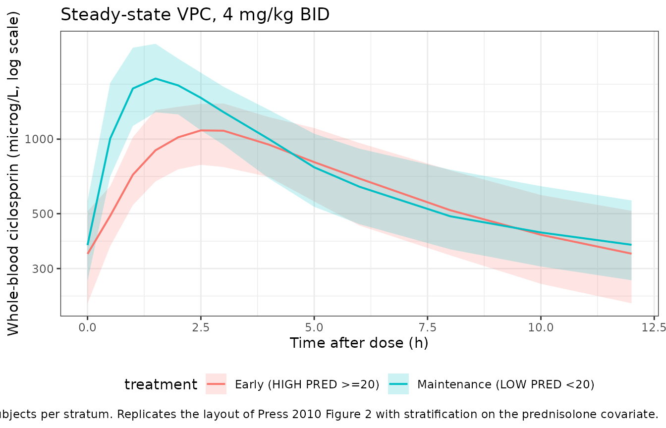
Typical-value contrast: prednisolone covariate effect
The typical-value profiles below isolate the covariate effect by removing inter-individual variability and using a single 76 kg subject. The HIGH-prednisolone profile shows the predicted 55% reduction in ka (later, lower peak) and 22% reduction in F (smaller AUC).
typical <- sim_typ |>
  dplyr::filter(!is.na(Cc), time >= ss_offset, id %in% c(1L, 101L)) |>
  dplyr::mutate(tad = time - ss_offset)

ggplot(typical, aes(x = tad, y = Cc, colour = treatment)) +
  geom_line(linewidth = 0.9) +
  geom_point(size = 1.5) +
  labs(
    x = "Time after dose (h)",
    y = "Whole-blood ciclosporin (microg/L)",
    title = "Typical-value steady-state profile, 4 mg/kg BID, WT = 76 kg",
    caption = paste(
      "Random effects zeroed; isolates the PRED_DOSE >= 20 mg/day",
      "covariate effect on ka (-55%) and F (-22%)."
    )
  ) +
  theme_bw() +
  theme(legend.position = "bottom")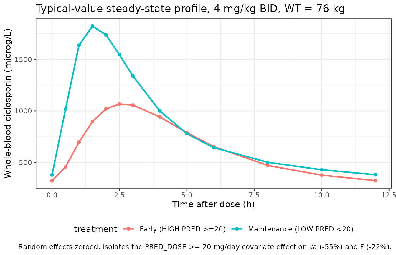
PKNCA validation
PKNCA is run on the steady-state dosing interval (the 9th BID interval, starting at 96 h). Cmax, Tmax, AUC over the dosing interval (AUClast), and average concentration (cav) are tabulated per stratum. The HIGH- prednisolone stratum should show a delayed Tmax, lower Cmax, and a proportionally lower AUC.
sim_nca <- sim |>
  dplyr::filter(!is.na(Cc), time >= ss_offset, time <= ss_offset + 12) |>
  dplyr::transmute(id, time = time - ss_offset, Cc, treatment)

# Time-zero anchor: pre-dose for the steady-state interval. At steady
# state Cc(0) is the trough concentration; using the simulated trough
# directly is appropriate here.
trough <- sim_nca |>
  dplyr::group_by(id, treatment) |>
  dplyr::summarise(Cc = min(Cc, na.rm = TRUE), .groups = "drop") |>
  dplyr::mutate(time = 0)

sim_nca <- dplyr::bind_rows(sim_nca, trough) |>
  dplyr::distinct(id, treatment, time, .keep_all = TRUE) |>
  dplyr::arrange(id, treatment, time)

dose_nca <- events |>
  dplyr::filter(evid == 1L, time == ss_offset) |>
  dplyr::transmute(id, time = 0, amt, treatment)

conc_obj <- PKNCA::PKNCAconc(
  data    = sim_nca,
  formula = Cc ~ time | treatment + id,
  concu   = "ug/L",
  timeu   = "h"
)

dose_obj <- PKNCA::PKNCAdose(
  data    = dose_nca,
  formula = amt ~ time | treatment + id,
  doseu   = "mg"
)

intervals <- data.frame(
  start   = 0,
  end     = 12,
  cmax    = TRUE,
  tmax    = TRUE,
  cmin    = TRUE,
  auclast = TRUE,
  cav     = TRUE
)

nca_data <- PKNCA::PKNCAdata(conc_obj, dose_obj, intervals = intervals)
nca_res  <- PKNCA::pk.nca(nca_data)
Comparison against the Press 2010 implied population
Press 2010 does not publish per-stratum NCA tables. The reference values below are derived from the model’s typical parameters and from the per-protocol AUC targets used for TDM (Methods page 580):
- Maintenance (LOW PRED): AUC0-12 = Dose * F / CL = (4 * 76) * 0.5 / 15 = 10.13 mgh/L = 10,130 microgh/L for the 4 mg/kg q12h starting regimen. The Press 2010 TDM target AUC0-12 was 5,400 microgh/L in the first 6 weeks (tapered down to 3,250 microgh/L thereafter), so the starting dose at steady state would be down-titrated by TDM to roughly half before reaching maintenance.
- Early post-transplant (HIGH PRED): ka is reduced by 55% and F by 22%; AUC0-12 is reduced proportionally to F (CL unchanged), giving an expected (0.5 * 0.78) / 0.5 = 0.78 ratio relative to the LOW-PRED stratum.
nca_tbl <- as.data.frame(nca_res$result) |>
  dplyr::filter(!is.na(PPORRES)) |>
  dplyr::group_by(treatment, PPTESTCD) |>
  dplyr::summarise(
    median = stats::median(PPORRES, na.rm = TRUE),
    q05    = stats::quantile(PPORRES, 0.05, na.rm = TRUE),
    q95    = stats::quantile(PPORRES, 0.95, na.rm = TRUE),
    .groups = "drop"
  ) |>
  dplyr::arrange(PPTESTCD, treatment)

knitr::kable(
  nca_tbl,
  caption = paste(
    "Steady-state NCA, 4 mg/kg q12h, by prednisolone stratum.",
    "Median and 5th / 95th percentiles over 100 virtual subjects per",
    "stratum. AUClast in microg*h/L, Cmax / Cmin / Cav in microg/L,",
    "Tmax in h."
  ),
  digits = 1
)| treatment | PPTESTCD | median | q05 | q95 |
|---|---|---|---|---|
| Early (HIGH PRED >=20) | auclast | 7851.8 | 5246.9 | 11141.9 |
| Maintenance (LOW PRED <20) | auclast | 10044.7 | 7133.5 | 12884.2 |
| Early (HIGH PRED >=20) | cav | 654.3 | 437.2 | 928.5 |
| Maintenance (LOW PRED <20) | cav | 837.1 | 594.5 | 1073.7 |
| Early (HIGH PRED >=20) | cmax | 1101.4 | 757.5 | 1517.5 |
| Maintenance (LOW PRED <20) | cmax | 1827.5 | 1251.7 | 2609.1 |
| Early (HIGH PRED >=20) | cmin | 343.7 | 197.5 | 581.8 |
| Maintenance (LOW PRED <20) | cmin | 373.0 | 236.8 | 594.8 |
| Early (HIGH PRED >=20) | tmax | 2.5 | 2.0 | 4.0 |
| Maintenance (LOW PRED <20) | tmax | 1.5 | 1.0 | 2.0 |
# Predicted ratio: HIGH-PRED / LOW-PRED AUC0-12 (analytical: 1 - 0.22 = 0.78)
auc_med <- nca_tbl |>
  dplyr::filter(PPTESTCD == "auclast") |>
  dplyr::select(treatment, median) |>
  tidyr::pivot_wider(names_from = treatment, values_from = median)

ratio <- as.numeric(auc_med[["Early (HIGH PRED >=20)"]]) /
         as.numeric(auc_med[["Maintenance (LOW PRED <20)"]])

cat(sprintf(
  "HIGH:LOW AUClast ratio = %.3f (analytic 1 - 0.22 = 0.780)\n",
  ratio
))
#> HIGH:LOW AUClast ratio = 0.782 (analytic 1 - 0.22 = 0.780)
The simulated HIGH:LOW ratio should sit close to the analytic 0.78 (F is reduced by 22% in the HIGH stratum; CL and Vc are unchanged).
Assumptions and deviations
-
Inter-occasion variability encoded as IIV. Press
2010 estimated the bioavailability random effect as inter-occasion
variability across sampling visits (Methods ‘Random effects’; Table 4
‘IOV bioavailability’). The rxode2 simulation API in nlmixr2lib does not
preserve a per-subject occasion structure, so this term is encoded as
IIV on
lfdepotwith the same variance (0.02). The marginal magnitude of bioavailability variability is preserved; the within-subject occasion-to-occasion structure is not. -
Threshold-form prednisolone covariate. Press 2010
reports the prednisolone effect as a binary contrast at the >= 20
mg/day threshold (Table 4 footnote b). The model uses the continuous
PRED_DOSEcolumn in the input data and forms the binary indicator insidemodel()(pred_high <- (PRED_DOSE >= 20)). Downstream users simulating the prednisolone taper should supply the actual daily prednisolone dose; the >= 20 threshold collapses the dose into the HIGH stratum used by the model. - No allometric scaling on Vp or Q. Press 2010 fits the allometric body-weight effect only to CL and Vc (Results ‘CsA pharmacokinetic model’); the peripheral volume Vp and intercompartmental clearance Q carry no covariate effect in the source paper and the packaged model reproduces this choice.
-
Residual error encoded as proportional in the linear
domain. Press 2010 Methods ‘Random effects’ uses additive error
on the log scale: log(Cij) = log(Cpredij) + eps with sigma^2 = 0.07.
This is equivalent to a proportional error in the linear domain at the
typical CV (sqrt(0.07) ~ 26%), so the packaged model uses
Cc ~ prop(propSd)withpropSd = 0.2646per the same precedent set byStorset_2014_tacrolimus.RandTerHeine_2018_everolimus.Rfor papers that state “additive on log scale”. - Cohort weight distribution approximated. Press 2010 reports weight range 49 - 140 kg and median 76 kg (Results page 581) but no full distribution. The virtual cohort draws weights from a log-normal centred at the median with SD = 0.22 on the log scale, reproducing the central 95% span; this is a simulation convenience and not a parameter of the model.
- Genetic polymorphisms not encoded. Press 2010 tested twelve SNPs in ABCB1, CYP3A4, CYP3A5, and PXR and reported no significant effect retained in the final model (Results ‘Genotype effects on PK’; Discussion). The packaged model therefore carries no pharmacogenetic covariate.