Docetaxel millidose and therapeutic dose (Heerma van Voss 2024)
Source:vignettes/articles/HeermavanVoss_2024_docetaxel.Rmd
HeermavanVoss_2024_docetaxel.RmdModel and source
- Citation: Heerma van Voss MR, Notohardjo J, van Dodewaard-de Jong J, Bloemendal HJ, ter Heine R. A sub-pharmacological test dose does not predict individual docetaxel exposure in prostate cancer patients. Cancer Chemother Pharmacol. 2024;94(3):437. doi:10.1007/s00280-024-04684-2.
- Article (open access): https://doi.org/10.1007/s00280-024-04684-2
- PubMed Central: https://pmc.ncbi.nlm.nih.gov/articles/PMC11420247/
Heerma van Voss et al. gave 29 men with prostate cancer an intravenous docetaxel test dose of 1000 ug (a “millidose”) one to seven days before their first therapeutic docetaxel infusion (75 mg/m^2 over 60 min) and asked whether the clearance of the test dose predicts the clearance of the therapeutic dose. The two datasets were fitted separately (Methods), each with a two-compartment linear model, so the paper contributes two independent models:
-
HeermavanVoss_2024_docetaxel_millidose– Two-compartment population PK model for a sub-pharmacological intravenous docetaxel test dose (millidose, 1000 ug bolus) in 29 men with prostate cancer, fitted separately from the therapeutic-dose data of the same patients. Clearance and inter-compartmental clearance scale with (WT/70)^0.75 and both volumes with (WT/70)^1 (fixed exponents). Inter-individual variability on CL and the peripheral volume; proportional residual error. -
HeermavanVoss_2024_docetaxel_therapeutic– Two-compartment population PK model for therapeutic intravenous docetaxel (75 mg/m^2 as a 60-minute infusion) in 29 men with prostate cancer, fitted separately from the millidose data of the same patients. Clearance and inter-compartmental clearance scale with (WT/70)^0.75 and both volumes with (WT/70)^1 (fixed exponents). Inter-individual variability on CL and the central volume; proportional residual error with a separate, larger proportional error for samples drawn during the infusion.
The individual clearances of the two doses were not correlated (Spearman’s rho = 0.02, Figure 1), so the two models carry independent random effects; the paper’s conclusion is that the millidose describes docetaxel PK at the population level (geometric mean ratio of clearance 1.44) but not in the individual patient.
Population
Thirty patients with prostate cancer treated with docetaxel 75 mg/m^2 as routine care at a general hospital in the Netherlands (2017-2020, EudraCT 2016-003785-77) were enrolled; one was excluded after an allergic reaction to the millidose, leaving 29 men (Table 1). Median age was 72 years (IQR 69-77), mean weight 85.5 kg (95% CI 69.4-100.8), mean body-surface area 2.02 m^2 (1.79-2.23), mean creatinine 90.9 umol/L and mean bilirubin 8.8 umol/L. Serum alpha-1-acid glycoprotein (AAG) was a median 0.73 g/L on the millidose day and 0.72 g/L on the therapeutic-dose day; it was tested on clearance and not retained. The mean therapeutic dose was 151.2 mg (133.6-168.0).
Plasma samples were drawn 0.25, 1, 2, 4, 6 and 8 h after the end of each dose (the millidose is a bolus; the therapeutic dose a 60-min infusion). Some therapeutic-dose samples were drawn during the infusion by mistake, and the therapeutic-dose model gives them their own proportional residual error.
The same information is available programmatically via
readModelDb("HeermavanVoss_2024_docetaxel_millidose")()$population.
Source trace
The per-parameter origin is recorded as an in-file comment next to
each ini() entry in
inst/modeldb/specificDrugs/HeermavanVoss_2024_docetaxel_millidose.R
and
inst/modeldb/specificDrugs/HeermavanVoss_2024_docetaxel_therapeutic.R.
| Equation / parameter | Millidose | Therapeutic dose | Source location |
|---|---|---|---|
Two-compartment linear disposition, IV input into
central
|
yes | yes | Results paragraph 1 |
lcl (CL at 70 kg, L/h) |
log(49.6) | log(34.6) | Table 2, Clearance |
lvc (Vc at 70 kg, L) |
log(6.7) | log(8.00) | Table 2, Central volume (millidose printed ‘6,7’) |
lq (Q at 70 kg, L/h) |
log(39.2) | log(4.63) | Table 2, Inter-compartmental clearance |
lvp (Vp at 70 kg, L) |
log(109) | log(22.2) | Table 2, Peripheral volume |
e_wt_cl (WT/70 exponent on CL and Q) |
fixed 0.75 | fixed 0.75 | Methods, allometric scaling |
e_wt_vc (WT/70 exponent on Vc and Vp) |
fixed 1 | fixed 1 | Methods, allometric scaling |
etalcl |
log(1 + 0.757^2) | log(1 + 0.617^2) | Table 2, IIV in clearance 75.7% / 61.7% |
etalvc |
– | log(1 + 0.692^2) | Table 2, IIV in central volume 69.2% |
etalvp |
log(1 + 0.765^2) | – | Table 2, IIV in peripheral volume 76.5% |
propSd |
0.370 | 0.471 | Table 2, Residual error 37.0% / 47.1% |
propSd_infusion (samples during infusion) |
– | 0.988 | Table 2, Residual error for samples drawn during infusion 98.8% |
Cc = central / vc * 1000 (ug/L) |
yes | yes | Methods (concentrations in ug/L; Supplement GOF captions) |
Virtual cohort
The observed data are not public. The virtual cohort draws weight and body-surface area independently from normal distributions whose mean and 2.5th-97.5th percentiles match Table 1 (the table’s “95% CI” is read as the spread of the patients, since a confidence interval of the mean of 29 values would be far narrower). The same 150 virtual patients receive the 1 mg millidose in one model and 75 mg/m^2 over 1 h in the other.
set.seed(20240901)
rxode2::rxSetSeed(20240901)

n_sub <- 150L
cohort <- tibble(
  id = seq_len(n_sub),
  WT = pmax(rnorm(n_sub, mean = 85.5, sd = (100.8 - 69.4) / (2 * 1.96)), 50),
  BSA = rnorm(n_sub, mean = 2.02, sd = (2.23 - 1.79) / (2 * 1.96))
)

# Dense grid for NCA plus the paper's sampling times (0.25-8 h after the end
# of each dose; the therapeutic infusion ends at 1 h).
obs_times <- sort(unique(c(seq(0, 2, by = 0.05), seq(2.25, 48, by = 0.25),
                           c(0.25, 1, 2, 4, 6, 8), 1 + c(0.25, 1, 2, 4, 6, 8))))

make_events <- function(cohort, dose_mg, tinf) {
  doses <- cohort |>
    mutate(time = 0, amt = dose_mg, evid = 1L, cmt = "central",
           rate = if (tinf > 0) amt / tinf else 0)
  obs <- tidyr::expand_grid(cohort, time = obs_times) |>
    mutate(amt = 0, evid = 0L, cmt = "central", rate = 0)
  bind_rows(doses, obs) |>
    mutate(TINF = tinf) |>
    arrange(id, time, desc(evid))
}

ev_milli <- make_events(cohort, dose_mg = 1, tinf = 0)
ev_ther <- make_events(cohort, dose_mg = 75 * cohort$BSA, tinf = 1)

stopifnot(
  !anyDuplicated(unique(ev_milli[, c("id", "time", "evid")])),
  !anyDuplicated(unique(ev_ther[, c("id", "time", "evid")])),
  abs(mean(ev_ther$amt[ev_ther$evid == 1]) / 151.2 - 1) < 0.05
)
Simulation
mod_milli <- readModelDb("HeermavanVoss_2024_docetaxel_millidose")
mod_ther <- readModelDb("HeermavanVoss_2024_docetaxel_therapeutic")

sim_milli <- rxode2::rxSolve(mod_milli, events = ev_milli, keep = "WT",
                             returnType = "data.frame") |>
  mutate(regimen = "Millidose (1 mg bolus)")
#> ℹ parameter labels from comments will be replaced by 'label()'
sim_ther <- rxode2::rxSolve(mod_ther, events = ev_ther, keep = "WT",
                            returnType = "data.frame") |>
  mutate(regimen = "Therapeutic (75 mg/m^2, 1 h)")
#> ℹ parameter labels from comments will be replaced by 'label()'
sim <- bind_rows(sim_milli, sim_ther)
Typical-value check against the reported geometric-mean clearance
Table 2 gives clearance for a 70 kg patient; the Results report the geometric mean of the individual (empirical Bayes) clearances, 57.9 L/h for the millidose and 40.3 L/h for the therapeutic dose. Scaling the Table 2 values to the cohort’s mean weight of 85.5 kg with the fixed 0.75 exponent reproduces both, which confirms the 70 kg reference and the allometric exponent. The ratio of the two typical clearances is the paper’s geometric mean ratio of 1.44.
cl70 <- c(
  millidose = exp(rxode2::rxode(mod_milli)$theta[["lcl"]]),
  therapeutic = exp(rxode2::rxode(mod_ther)$theta[["lcl"]])
)
#> ℹ parameter labels from comments will be replaced by 'label()'
#> ℹ parameter labels from comments will be replaced by 'label()'
cl_typ <- cl70 * (85.5 / 70)^0.75
tab_cl <- tibble(
  Dose = c("Millidose", "Therapeutic dose"),
  `CL at 70 kg (L/h)` = unname(cl70),
  `CL at 85.5 kg (L/h)` = unname(cl_typ),
  `Reported geometric mean (L/h)` = c(57.9, 40.3)
) |>
  mutate(`Difference (%)` = 100 * (`CL at 85.5 kg (L/h)` /
                                     `Reported geometric mean (L/h)` - 1))
knitr::kable(tab_cl, digits = 2,
caption = "Table 2 clearance scaled to the mean weight vs. the reported geometric mean.")| Dose | CL at 70 kg (L/h) | CL at 85.5 kg (L/h) | Reported geometric mean (L/h) | Difference (%) |
|---|---|---|---|---|
| Millidose | 49.6 | 57.63 | 57.9 | -0.47 |
| Therapeutic dose | 34.6 | 40.20 | 40.3 | -0.25 |
stopifnot(
  all(abs(tab_cl$`Difference (%)`) < 2),
  abs(cl70[["millidose"]] / cl70[["therapeutic"]] - 1.44) < 0.02
)
The individual clearances of the simulated cohort centre on the same values. Their spread includes the weight effect as well as the inter-individual variability; the paper’s geometric CVs of the empirical Bayes estimates (78.6% and 60.7%) are shown for orientation only, since empirical Bayes estimates shrink towards the typical value.
cl_ind <- sim |>
  group_by(regimen, id) |>
  summarise(cl = first(cl), .groups = "drop") |>
  group_by(regimen) |>
  summarise(
    `Geometric mean CL (L/h)` = exp(mean(log(cl))),
    `Geometric CV (%)` = 100 * sqrt(exp(var(log(cl))) - 1),
    .groups = "drop"
  ) |>
  mutate(`Reported geometric mean (L/h)` = c(57.9, 40.3),
         `Reported geometric CV (%)` = c(78.6, 60.7))
knitr::kable(cl_ind, digits = 1,
caption = "Simulated individual clearance vs. the reported empirical Bayes summaries.")| regimen | Geometric mean CL (L/h) | Geometric CV (%) | Reported geometric mean (L/h) | Reported geometric CV (%) |
|---|---|---|---|---|
| Millidose (1 mg bolus) | 60.3 | 77.3 | 57.9 | 78.6 |
| Therapeutic (75 mg/m^2, 1 h) | 42.5 | 62.4 | 40.3 | 60.7 |
Concentration-time profiles
The supplement shows prediction-corrected VPCs for both datasets. The plot below shows the 5th, 50th and 95th percentiles of the simulated concentrations over the paper’s 8 h sampling window (millidose) and 9 h from the start of the infusion (therapeutic dose), for comparison with those panels. Both models have a very fast distribution phase (initial half-life of a few minutes), so the first sample after each dose is highly sensitive to its exact timing. The simulated millidose median is about 7 ug/L at 0.25 h and about 1 ug/L at 1 h, with a 95th percentile near the supplement’s upper observed percentile at 0.25 h (about 20 ug/L); the observed median at 0.25 h in the prediction- corrected VPC is lower, about 2-3 ug/L. The simulated therapeutic median is about 1000 ug/L 15 min after the end of the infusion, falling to about 100 ug/L by 2 h.
sim |>
  filter(time > 0, time <= 9) |>
  group_by(regimen, time) |>
  summarise(
    Q05 = quantile(Cc, 0.05), Q50 = median(Cc), Q95 = quantile(Cc, 0.95),
    .groups = "drop"
  ) |>
  ggplot(aes(time, Q50)) +
  geom_ribbon(aes(ymin = Q05, ymax = Q95), alpha = 0.25) +
  geom_line() +
  facet_wrap(~regimen, ncol = 1, scales = "free_y") +
  scale_y_log10() +
  labs(x = "Time after the start of dosing (h)",
       y = "Docetaxel concentration (ug/L)",
       caption = paste("Median and 90% prediction interval of 150 virtual patients;",
                       "compare the VPCs in the supplement of Heerma van Voss 2024."))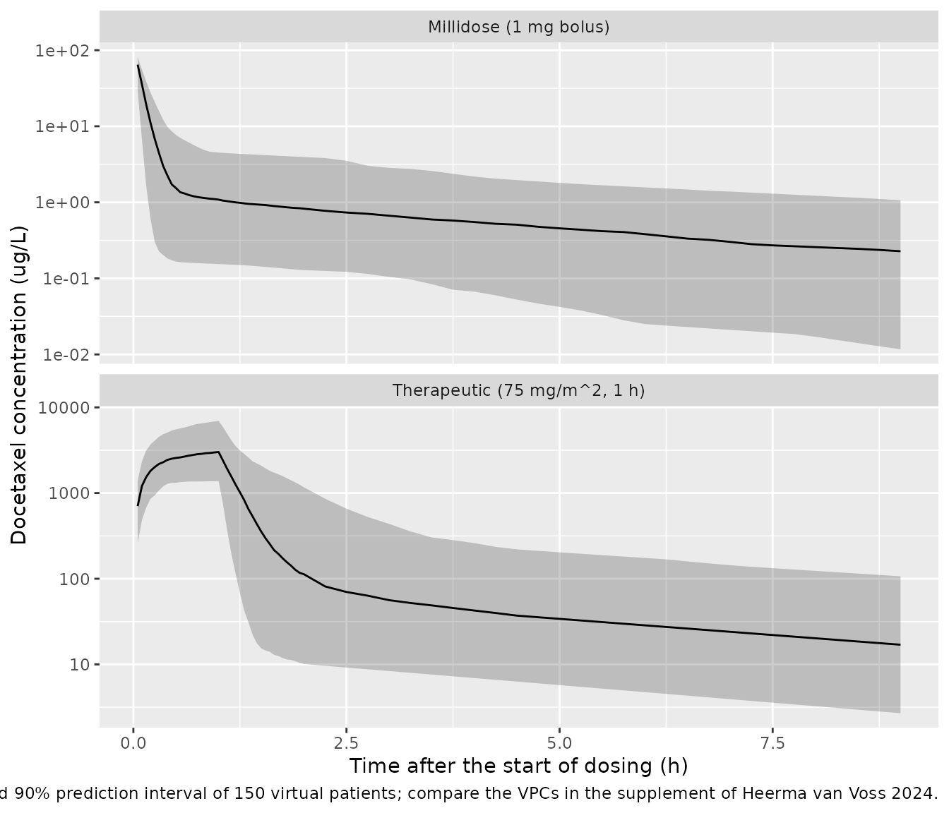
Dose-normalising the typical-value profiles shows how differently the two fits distribute the drug. The therapeutic-dose model has the lower clearance (so the larger AUC per mg), but most of that exposure falls during the infusion; the millidose model’s large, rapidly equilibrating peripheral volume (109 L vs 22.2 L at 70 kg) keeps its dose-normalised concentration above the therapeutic one from about 2 h onwards.
typ_ev <- function(dose_mg, tinf) {
  make_events(tibble(id = 1L, WT = 85.5, BSA = 2.02), dose_mg, tinf)
}
typ <- bind_rows(
  rxode2::rxSolve(rxode2::zeroRe(mod_milli), events = typ_ev(1, 0),
                  returnType = "data.frame") |>
    mutate(regimen = "Millidose (1 mg bolus)", Cn = Cc / 1),
  rxode2::rxSolve(rxode2::zeroRe(mod_ther), events = typ_ev(151.5, 1),
                  returnType = "data.frame") |>
    mutate(regimen = "Therapeutic (151.5 mg, 1 h)", Cn = Cc / 151.5)
)
#> ℹ parameter labels from comments will be replaced by 'label()'
#> ℹ omega/sigma items treated as zero: 'etalcl', 'etalvp'
#> ℹ parameter labels from comments will be replaced by 'label()'
#> Warning: No sigma parameters in the model
#> ℹ omega/sigma items treated as zero: 'etalcl', 'etalvc'
typ |>
  filter(time > 0, time <= 12) |>
  ggplot(aes(time, Cn, colour = regimen)) +
  geom_line() +
  scale_y_log10() +
  labs(x = "Time after the start of dosing (h)",
       y = "Dose-normalised concentration (ug/L per mg)", colour = NULL,
       caption = "Typical 85.5 kg patient (Table 1 mean weight and BSA).") +
  theme(legend.position = "bottom")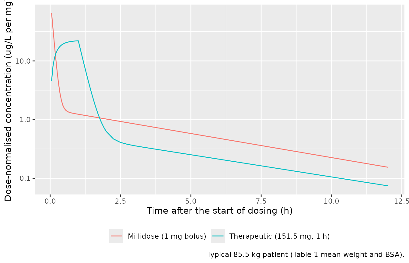
PKNCA validation
The paper reports no NCA. Because exposure after an intravenous dose
is AUC = dose / CL, the reported geometric mean clearances
give a reference AUC: 1 mg / 57.9 L/h = 17.3 ugh/L for the millidose
and 151.2 mg / 40.3 L/h = 3752 ugh/L for the mean therapeutic dose.
PKNCA is run on the simulated profiles (0-48 h, about ten terminal
half-lives) and its median AUC compared with these values.
conc <- sim |>
  filter(!is.na(Cc)) |>
  mutate(Cc = pmax(Cc, 0)) |>
  select(id, time, Cc, regimen)
doses <- bind_rows(
  ev_milli |> filter(evid == 1) |> mutate(regimen = "Millidose (1 mg bolus)", duration = 0),
  ev_ther |> filter(evid == 1) |> mutate(regimen = "Therapeutic (75 mg/m^2, 1 h)", duration = 1)
) |>
  select(id, time, amt, regimen, duration)

conc_obj <- PKNCA::PKNCAconc(conc, Cc ~ time | regimen + id)
dose_obj <- PKNCA::PKNCAdose(doses, amt ~ time | regimen + id,
                             route = "intravascular", duration = "duration")
intervals <- data.frame(start = 0, end = Inf, cmax = TRUE, tmax = TRUE,
                        aucinf.obs = TRUE, half.life = TRUE)
nca_res <- PKNCA::pk.nca(PKNCA::PKNCAdata(conc_obj, dose_obj, intervals = intervals))

published <- tibble::tribble(
  ~regimen, ~aucinf.obs,
  "Millidose (1 mg bolus)", 1000 / 57.9,
  "Therapeutic (75 mg/m^2, 1 h)", 151.2 * 1000 / 40.3
)
cmp <- nlmixr2lib::ncaComparisonTable(
  simulated = nca_res,
  reference = published,
  by = "regimen",
  units = c(cmax = "ug/L", tmax = "h", aucinf.obs = "ug*h/L", half.life = "h"),
  tolerance_pct = 20
)
knitr::kable(cmp, caption = paste(
  "Simulated NCA vs. the AUC implied by the reported geometric mean clearance.",
  "* differs from reference by >20%."
))| NCA parameter | regimen | Reference | Simulated | % diff |
|---|---|---|---|---|
| AUC0-∞ (obs) (ug*h/L) | Millidose (1 mg bolus) | 17.3 | 17.4 | +0.9% |
| AUC0-∞ (obs) (ug*h/L) | Therapeutic (75 mg/m^2, 1 h) | 3750 | 3500 | -6.6% |
The same-subject check is tighter: PKNCA’s AUC for each virtual patient must equal that patient’s dose divided by their own clearance, up to the trapezoidal and extrapolation error of the grid.
auc_chk <- as.data.frame(nca_res) |>
  filter(PPTESTCD == "aucinf.obs") |>
  select(id, regimen, auc = PPORRES) |>
  left_join(sim |> group_by(regimen, id) |> summarise(cl = first(cl), .groups = "drop"),
            by = c("regimen", "id")) |>
  left_join(doses |> select(id, regimen, amt), by = c("regimen", "id")) |>
  mutate(pct_diff = 100 * (auc / (amt / cl * 1000) - 1))

auc_chk |>
  group_by(regimen) |>
  summarise(`Median % difference` = median(pct_diff),
            `90th percentile of absolute % difference` = quantile(abs(pct_diff), 0.9),
            .groups = "drop") |>
knitr::kable(digits = 2, caption = "PKNCA AUC vs. dose / individual CL.")| regimen | Median % difference | 90th percentile of absolute % difference |
|---|---|---|
| Millidose (1 mg bolus) | 0.09 | 0.23 |
| Therapeutic (75 mg/m^2, 1 h) | -0.07 | 0.22 |
Assumptions and deviations
-
IIV scale. Table 2 reports inter-individual
variability in percent without stating the conversion. The maintainers
read the percentages as coefficients of variation of a log-normal
parameter,
omega^2 = log(1 + CV^2). The alternative reading (omega = CV / 100) gives about 12% larger standard deviations on the log scale; the paper’s reported geometric CVs of the individual clearances (78.6% and 60.7%, which include the weight effect and shrinkage) do not discriminate between the two. - Residual error. Table 2 percentages are used as proportional standard deviations (0.370, 0.471, 0.988).
-
Millidose central volume. Table 2 prints
6,7, read as 6.7 L (decimal comma). -
Samples during the infusion. The therapeutic-dose
model applies the 98.8% proportional error to samples taken while the
infusion is running, detected as
tad(central) < TINF;TINFmust be supplied as the infusion duration in hours (1 h in the study). The structural model is the same for every sample. - Independent random effects across the two models. The paper fitted the two datasets separately and found no correlation between the individual clearances (Figure 1), so the two library models carry unrelated etas. A simulation of the same patient under both doses (as above) draws them independently.
- Virtual cohort. Weight and BSA were drawn independently from normal distributions matching Table 1; the paper does not report their correlation or height. Age, creatinine, bilirubin and AAG do not enter either model.
- Reference AUC. The paper reports no NCA; the reference AUC in the comparison table is dose / reported geometric mean clearance, not a measured value.
- No correction notice affecting the model was found as of 2026-10-30 (the 2024-08-31 revision corrected an author’s name only).