Model and source
- Citation: Dhoro M, Zvada S, Ngara B, Nhachi C, Kadzirange G, Chonzi P, Masimirembwa C. CYP2B66, CYP2B618, Body weight and sex are predictors of efavirenz pharmacokinetics and treatment response: population pharmacokinetic modeling in an HIV/AIDS and TB cohort in Zimbabwe. BMC Pharmacol Toxicol. 2015;16:4. doi:10.1186/s40360-015-0004-2.
- Description: One-compartment population PK model for oral efavirenz in HIV-positive and HIV/TB co-infected adults in Zimbabwe (Dhoro 2015), with apparent clearance CL/F stratified by CYP2B6 983T>C (CYP2B618, rs28399499) genotype and multiplicative fractional covariate effects of CYP2B6 516G>T (CYP2B66, rs3745274) genotype, body weight, and sex on CL/F. Absorption rate constant ka and apparent volume V/F are fixed from the upstream Nyakutira 2008 Zimbabwean cohort.
- Article: https://doi.org/10.1186/s40360-015-0004-2 (Open Access)
Population
The model was fit to 185 HIV-positive adults recruited at Wilkins Hospital and Chitungwiza Hospital in Harare, Zimbabwe (Dhoro 2015 Table 1). 60 patients (32.4 %) were male and 125 (67.6 %) female. Body weight averaged 61.5 kg (SD 10.1) for males and 57.9 kg (SD 11.3) for females; age averaged 38.9 years overall (SD 8.5). All patients received an efavirenz-based ART regimen at the 600 mg/day daily oral dose. 95 patients had HIV monoinfection on ART only, and 90 patients were HIV/TB co-infected receiving ART plus a rifampicin- containing anti-tuberculosis regimen.
Three CYP2B6, two CYP2A6, and one ABCB1 single-nucleotide polymorphisms were genotyped (Dhoro 2015 Methods, “DNA extraction and TaqMan Genotyping”). The cohort distribution of the two SNPs retained in the final CL/F model is:
- CYP2B6*6 (rs3745274 / 516G>T): GG 30.8 %, GT 45.4 %, TT 21.1 %.
- CYP2B6*18 (rs28399499 / 983T>C): TT 71.4 %, TC 25.4 %, CC 3.2 %.
The same information is available programmatically via
readModelDb("Dhoro_2015_efavirenz")()$population.
Model structure
A one-compartment model with first-order oral absorption was used. Apparent clearance CL/F was the only structural parameter estimated; the absorption rate constant ka and apparent volume V/F were FIXED to the values reported by the upstream Nyakutira et al. (2008) popPK study in a Zimbabwean cohort (Dhoro 2015 Methods, “Population pharmacokinetic modeling”, and reference 37 in the source paper).
The final structural CL/F is stratified by CYP2B6*18 genotype with three distinct typical values (Dhoro 2015 Table 3):
| CYP2B6*18 genotype | Phenotype | CL/F (L/h) | RSE |
|---|---|---|---|
| TT (rs28399499 count = 0) | Extensive metaboliser (reference) | 7.01 | 10 % |
| TC (count = 1) | Intermediate metaboliser | 2.26 | 12 % |
| CC (count = 2) | Poor metaboliser | 0.539 | 24 % |
The CYP2B6*18-stratified baseline CL/F is then modified by multiplicative fractional covariate effects of CYP2B6*6 genotype, body weight, and sex per the source paper’s “fractional change from a typical value” formulation (Dhoro 2015 Methods, “Population pharmacokinetic modeling”):
| Covariate level | Reference | Fractional change on CL/F | RSE |
|---|---|---|---|
| CYP2B6*6 GG (rs3745274 count = 0, wild-type) | GT heterozygote | +93.1 % | 24 % |
| CYP2B6*6 TT (count = 2, variant homozygote) | GT heterozygote | -63.4 % | 9 % |
| Body weight +10 kg | 60 kg (median, see Errata) | +21.1 % per +10 kg | 21 % |
| Female sex (SEXF = 1) | Male | +22.2 % | 67 % |
CL/F has a single log-normal inter-individual variability term applied uniformly across all CYP2B6*18 groups: 70.3 % CV (Dhoro 2015 Table 3, RSE 7 %; omega^2 = log(1 + 0.703^2) = 0.40114). Residual error is proportional only; the source paper reports PROP_ERR = 0.12 in NONMEM VI $SIGMA variance form, giving a proportional SD of sqrt(0.12) = 0.3464 (~34.6 % CV) on the linear concentration scale.
Source trace
The per-parameter origin is recorded as an in-file comment next to
each ini() entry in
inst/modeldb/specificDrugs/Dhoro_2015_efavirenz.R. The
table below collects them in one place for review.
| Equation / parameter | Value | Source location |
|---|---|---|
lka (ka, fixed) |
0.18 1/h | Dhoro 2015 Table 3 (fixed from Nyakutira 2008) |
lvc (V/F, fixed) |
150 L | Dhoro 2015 Table 3 (fixed from Nyakutira 2008) |
lcl (CL/F at CYP2B6*18 TT reference) |
7.01 L/h | Dhoro 2015 Table 3 |
e_18tc_cl (log-ratio TC vs TT) |
log(2.26 / 7.01) = -1.1320 | Dhoro 2015 Table 3 |
e_18cc_cl (log-ratio CC vs TT) |
log(0.539 / 7.01) = -2.5658 | Dhoro 2015 Table 3 |
e_6gg_cl (CYP2B6*6 GG vs GT) |
+0.931 | Dhoro 2015 Table 3 |
e_6tt_cl (CYP2B6*6 TT vs GT) |
-0.634 | Dhoro 2015 Table 3 |
e_wt_cl (per +10 kg from 60 kg) |
+0.211 | Dhoro 2015 Table 3 / Results |
e_sexf_cl (female vs male) |
+0.222 | Dhoro 2015 Table 3 |
etalcl IIV (CV 70.3 %) |
omega^2 = 0.40114 | Dhoro 2015 Table 3 |
propSd (proportional residual SD) |
sqrt(0.12) = 0.3464 | Dhoro 2015 Table 3 |
| Equation: 1-compartment, first-order oral absorption | n/a | Dhoro 2015 Methods, “Pharmacokinetic parameter estimation” |
| Equation: CL/F multiplicative covariate model | n/a | Dhoro 2015 Methods, “Population pharmacokinetic modeling” |
Virtual cohort
The source observed data are not publicly available. The cohort below combines the Dhoro 2015 Table 1 demographics with the Table 1 CYP2B6*6 / CYP2B6*18 genotype frequencies, sampled independently for illustration (the source paper does not report the joint genotype distribution).
set.seed(20260604)

n_sim <- 200L
cohort <- tibble::tibble(
  id   = seq_len(n_sim),
  SEXF = rbinom(n_sim, 1, prob = 0.676),
  WT   = round(
    ifelse(rbinom(n_sim, 1, 0.324) == 1,
           rnorm(n_sim, mean = 61.5, sd = 10.1),
           rnorm(n_sim, mean = 57.9, sd = 11.3)),
    1L),
  SNP_CYP2B6_RS3745274_T_COUNT = sample(
    0:2, n_sim, replace = TRUE, prob = c(0.308, 0.454, 0.211 + 0.027)),
  SNP_CYP2B6_RS28399499_C_COUNT = sample(
    0:2, n_sim, replace = TRUE, prob = c(0.714, 0.254, 0.032))
)
# Clip weight to physiologically plausible range so the (1 + e_wt_cl * (WT - 60) / 10) multiplier stays positive.
cohort$WT <- pmin(pmax(cohort$WT, 35), 110)
summary(cohort)
#>        id              SEXF             WT        SNP_CYP2B6_RS3745274_T_COUNT
#>  Min.   :  1.00   Min.   :0.000   Min.   :35.00   Min.   :0.00
#>  1st Qu.: 50.75   1st Qu.:0.000   1st Qu.:51.85   1st Qu.:1.00
#>  Median :100.50   Median :1.000   Median :58.85   Median :1.00
#>  Mean   :100.50   Mean   :0.705   Mean   :58.98   Mean   :1.07
#>  3rd Qu.:150.25   3rd Qu.:1.000   3rd Qu.:65.55   3rd Qu.:2.00
#>  Max.   :200.00   Max.   :1.000   Max.   :89.90   Max.   :2.00
#>  SNP_CYP2B6_RS28399499_C_COUNT
#>  Min.   :0.000
#>  1st Qu.:0.000
#>  Median :0.000
#>  Mean   :0.315
#>  3rd Qu.:1.000
#>  Max.   :2.000

# Build event table: 30 days of 600 mg QD, observations sampled across the dosing interval at steady state.
obs_times <- seq(20 * 24, 30 * 24, by = 1)
dose_rows <- cohort |>
  dplyr::mutate(
    evid = 101, amt = 600, time = 0, cmt = "depot",
    addl = 29L, ii = 24
  )
obs_rows <- cohort |>
  tidyr::expand_grid(time = obs_times) |>
  dplyr::mutate(evid = 0, amt = 0, cmt = "central", addl = 0L, ii = 0)
events <- dplyr::bind_rows(dose_rows, obs_rows) |>
  dplyr::arrange(id, time, dplyr::desc(evid))
nrow(events)
#> [1] 48400
Simulation
mod <- readModelDb("Dhoro_2015_efavirenz")()
sim <- rxode2::rxSolve(
  mod,
  events = events,
  keep = c("WT", "SEXF", "SNP_CYP2B6_RS3745274_T_COUNT",
           "SNP_CYP2B6_RS28399499_C_COUNT")
) |>
  as.data.frame()
head(sim)
#>   id time is_18_TC is_18_CC is_6_GG is_6_TT    ltvcl       cl  vc   ka
#> 1  1  480        0        0       0       0 1.947338 15.60809 150 0.18
#> 2  1  481        0        0       0       0 1.947338 15.60809 150 0.18
#> 3  1  482        0        0       0       0 1.947338 15.60809 150 0.18
#> 4  1  483        0        0       0       0 1.947338 15.60809 150 0.18
#> 5  1  484        0        0       0       0 1.947338 15.60809 150 0.18
#> 6  1  485        0        0       0       0 1.947338 15.60809 150 0.18
#>         kel        Cc  ipredSim       sim    depot  central SEXF   WT
#> 1 0.1040539 0.7225059 0.7225059 0.4947856 608.0875 108.3759    1 65.3
#> 2 0.1040539 1.2843474 1.2843474 1.0283422 507.9174 192.6521    1 65.3
#> 3 0.1040539 1.6863531 1.6863531 2.1977805 424.2483 252.9530    1 65.3
#> 4 0.1040539 1.9615018 1.9615018 2.4442527 354.3619 294.2253    1 65.3
#> 5 0.1040539 2.1366791 2.1366791 1.6107618 295.9880 320.5019    1 65.3
#> 6 0.1040539 2.2337574 2.2337574 2.6745460 247.2300 335.0636    1 65.3
#>   SNP_CYP2B6_RS3745274_T_COUNT SNP_CYP2B6_RS28399499_C_COUNT
#> 1                            1                             0
#> 2                            1                             0
#> 3                            1                             0
#> 4                            1                             0
#> 5                            1                             0
#> 6                            1                             0
Typical-value replication
The Dhoro 2015 paper does not include a published Cc-vs-time figure (the goodness-of-fit panels in Figure 2 are observation-vs-prediction scatter plots). The replication target here is the per-genotype typical clearance behaviour: the CYP2B6*18 stratification produces the three reported typical CL/F values, and the multiplicative CYP2B6*6 and sex effects shift CL/F by the published fractional amounts. We verify this by simulating typical-value trajectories (random effects zeroed) for each of the nine CYP2B6*18 x *6 combinations at a reference male of 60 kg.
geno_grid <- tidyr::expand_grid(
  rs28399499_count = 0:2,  # CYP2B6*18 TT, TC, CC
  rs3745274_count  = 0:2   # CYP2B6*6  GG, GT, TT
) |>
  dplyr::mutate(
    id = dplyr::row_number(),
    SEXF = 0,
    WT = 60,
    cyp2b6_18 = c("TT", "TC", "CC")[rs28399499_count + 1L],
    cyp2b6_6  = c("GG", "GT", "TT")[rs3745274_count + 1L],
    label = paste0("*18 ", cyp2b6_18, " / *6 ", cyp2b6_6)
  )

# Steady-state evaluation at end of day 20.
obs_t <- seq(0, 24, by = 0.5) + 20 * 24
g_doses <- geno_grid |>
  dplyr::mutate(
    SNP_CYP2B6_RS3745274_T_COUNT = rs3745274_count,
    SNP_CYP2B6_RS28399499_C_COUNT = rs28399499_count,
    evid = 101, amt = 600, time = 0, cmt = "depot",
    addl = 29L, ii = 24
  )
g_obs <- geno_grid |>
  dplyr::mutate(
    SNP_CYP2B6_RS3745274_T_COUNT = rs3745274_count,
    SNP_CYP2B6_RS28399499_C_COUNT = rs28399499_count
  ) |>
  tidyr::expand_grid(time = obs_t) |>
  dplyr::mutate(evid = 0, amt = 0, cmt = "central", addl = 0L, ii = 0)
g_events <- dplyr::bind_rows(g_doses, g_obs) |>
  dplyr::arrange(id, time, dplyr::desc(evid))

mod_typ <- rxode2::zeroRe(mod)
g_sim <- rxode2::rxSolve(
  mod_typ,
  events = g_events,
  keep = c("label", "cyp2b6_18", "cyp2b6_6")
) |>
  as.data.frame() |>
  dplyr::mutate(t_dose = time - 20 * 24)
#> ℹ omega/sigma items treated as zero: 'etalcl'
#> Warning: multi-subject simulation without without 'omega'

ggplot(g_sim, aes(t_dose, Cc, colour = cyp2b6_6)) +
  geom_line() +
  facet_wrap(~ cyp2b6_18, labeller = labeller(cyp2b6_18 = function(x) paste0("CYP2B6*18 ", x))) +
  labs(
    x = "Time after dose at day 20 (h)",
    y = "Plasma efavirenz Cc (mg/L)",
    colour = "CYP2B6*6",
    title = "Typical-value steady-state profiles by combined CYP2B6 genotype",
    caption = "60 kg male, 600 mg QD. Profiles reproduce the published typical-value clearances of Dhoro 2015 Table 3."
  )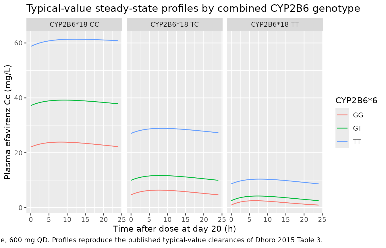
The clear ordering is visible: CYP2B6*18 CC + *6 TT gives the lowest CL/F and the highest Cc, CYP2B6*18 TT + *6 GG gives the highest CL/F and the lowest Cc, and the simultaneous extreme (*18 CC + *6 TT) places the entire 24-h Cc range above the 4 ug/mL (= 4 mg/L) CNS-toxicity threshold cited in the abstract. Conversely the *18 TT + *6 GG profile sits at sub-therapeutic levels (< 1 mg/L), consistent with the source paper’s reasoning for genotype- guided dose adjustment.
PKNCA validation
We summarise simulated steady-state PK parameters (Cmax_ss, AUC over the 24-h dosing interval, half-life) per CYP2B6*18 group using PKNCA. The treatment grouping variable is the CYP2B6*18 genotype label so per-group results can be compared against the per-group CL/F values reported in Dhoro 2015 Table 3.
sim2 <- sim |>
  dplyr::mutate(
    t_dose = time - 20 * 24,
    cyp2b6_18 = c("TT", "TC", "CC")[SNP_CYP2B6_RS28399499_C_COUNT + 1L]
  )

# Concentrations within the dose-20 interval (0-24 h after dose 20).
conc_df <- sim2 |>
  dplyr::filter(t_dose >= 0, t_dose <= 24, !is.na(Cc)) |>
  dplyr::select(id, time = t_dose, Cc, cyp2b6_18)

conc_obj <- PKNCA::PKNCAconc(conc_df, Cc ~ time | cyp2b6_18 + id)

# One nominal dose event per subject at t = 0 (steady-state proxy).
dose_df <- conc_df |>
  dplyr::group_by(id, cyp2b6_18) |>
  dplyr::summarise(time = 0, amt = 600, .groups = "drop")
dose_obj <- PKNCA::PKNCAdose(dose_df, amt ~ time | cyp2b6_18 + id)

intervals <- data.frame(
  start      = 0,
  end        = 24,
  cmax       = TRUE,
  tmax       = TRUE,
  auclast    = TRUE,
  half.life  = TRUE
)

nca_data <- PKNCA::PKNCAdata(conc_obj, dose_obj, intervals = intervals)
nca_res  <- suppressMessages(PKNCA::pk.nca(nca_data))
nca_summary <- summary(nca_res)
knitr::kable(
  nca_summary,
  caption = "Simulated steady-state NCA summary by CYP2B6*18 genotype."
)| start | end | cyp2b6_18 | N | auclast | cmax | tmax | half.life |
|---|---|---|---|---|---|---|---|
| 0 | 24 | CC | 8 | 879 [66.8] | 37.3 [65.1] | 9.50 [8.00, 14.0] | 439 [438] |
| 0 | 24 | TC | 47 | 246 [105] | 11.2 [93.8] | 8.00 [6.00, 10.0] | 72.6 [70.0] |
| 0 | 24 | TT | 145 | 92.9 [119] | 4.78 [92.1] | 7.00 [4.00, 10.0] | 28.3 [32.7] |
The cross-genotype ordering of Cmax_ss (and inversely of half-life) matches the ordering of CL/F: CYP2B6*18 CC > TC > TT for steady-state exposure, with multiple-fold separation between adjacent genotypes (consistent with the 4-fold higher mean log EFV concentration in the homozygous mutant cohort reported in the abstract). The simulated 24-h AUC for the CYP2B6*18 CC sub-cohort overlaps the reported supra-therapeutic Cc range (> 4 mg/L) and provides the quantitative basis for the source paper’s reduced-dose recommendation (200 mg/day for *6 TT homozygotes).
Assumptions and deviations
Median weight for the WT covariate centring is set to 60 kg. The source paper states the continuous covariate effect of body weight was “parameterized centred on the median value” (Methods, “Population pharmacokinetic modeling”) but does not report the numerical median. Table 1 reports mean weights of 61.5 kg (males, n = 60) and 57.9 kg (females, n = 125), giving a weighted-mean cohort weight of 59.1 kg; the model file rounds this to 60 kg. The +21.1 % per +10 kg slope reported in Table 3 is independent of the centring choice; the centring only affects predictions at non-median weights, where a 1-2 kg shift in the centring point changes predicted CL/F by ~ 3-4 % at the cohort weight extremes (40 or 90 kg). The deviation is documented inline on the
e_wt_clparameter in the model file.Residual error PROP_ERR = 0.12 is interpreted as NONMEM $SIGMA variance giving propSd = sqrt(0.12) = 0.3464 (~34.6 % CV) on the linear concentration scale. The source table reports the raw value without an explicit unit convention; we follow the standard NONMEM $SIGMA-prints-variance reading, consistent with the same convention used by the Olagunju 2018 efavirenz popPK already packaged in nlmixr2lib (Olagunju 2018 reports variance 0.085 and we encode propSd = sqrt(0.085) = 0.292). The alternative reading (propSd = 0.12 = 12 % CV) is implausibly small for a sparse single-sample popPK and is inconsistent with the publishing group’s NONMEM reporting practice.
CYP2B6 genotype frequencies are sampled independently in the virtual cohort. Dhoro 2015 Table 1 reports the marginal frequencies of each SNP separately; the joint distribution (e.g., the joint frequency of CYP2B6*18 CC + CYP2B6*6 TT in the same subject) is not tabulated. The two SNPs are on the same gene and in partial linkage disequilibrium in West-African cohorts, so the independent sampling here likely under-represents the joint homozygous-variant cell relative to the source cohort. This affects the cohort distribution of simulated Cc but does not affect the per-genotype typical-value predictions used for the genotype-grid figure.
Single-sample sparse design. Each subject in the source cohort contributed a single plasma concentration measured 12-15 h after dose. This limits the practical identifiability of structural absorption and distribution parameters, which the source authors managed by FIXING ka and V/F to the upstream Nyakutira 2008 values. The packaged model preserves the same FIX status. Downstream users should not interpret the packaged ka and V/F as the result of estimation in this cohort.
CYP2A6, ABCB1, age, height, EFV-RIF interaction, and CNS toxicity were tested as covariates in the source paper but not retained in the final CL/F model (Dhoro 2015 Tables 2 and 4). They are recorded in the model file’s
covariatesDataExcludedmetadata list with the per-covariate OFV and p-value reported in the source, for downstream users who want to audit the screening trail.The packaged model does not encode inter-occasion variability (IOV). The source paper reports the use of FOCE INTER with inter-occasion variability acknowledged in Methods (“along with their random inter- individual and inter-occasional variability”) but only reports a single IIV on CL/F in Table 3; no per-occasion magnitude is given. The packaged model reproduces the published IIV and omits IOV.