Aripiprazole (Zhang 2024)
Source:vignettes/articles/Zhang_2024_aripiprazole.Rmd
Zhang_2024_aripiprazole.RmdModel and source
- Citation: Zhang C, Jiang L, Hu K, Zhang Y-J, Han J, Chen J, Bulubu, Dong B, Shi H-Z, He S-M, Yu T-T, Chen X, Wang D-D. Drug-drug interaction and initial dosage optimization of aripiprazole in patients with schizophrenia based on population pharmacokinetics. Front Psychiatry. 2024 Jun 18;15:1377268. doi:10.3389/fpsyt.2024.1377268. The fixed absorption rate constant ka = 1.06 1/h is Zhang 2024 reference 14, Kim JR, Seo HB, Cho JY, et al. Population pharmacokinetic modelling of aripiprazole and its active metabolite, dehydroaripiprazole, in psychiatric patients. Br J Clin Pharmacol. 2008;66(6):802-810. doi:10.1111/j.1365-2125.2008.03223.x; see modellib(‘Kim_2008_aripiprazole’).
- Description: One-compartment first-order absorption population PK model for aripiprazole in Chinese adults with schizophrenia (Zhang 2024), built from routine therapeutic-drug-monitoring trough concentrations. Apparent oral clearance is allometrically scaled on body weight (exponent 0.75, 70 kg reference) and reduced 28.6% by concomitant fluoxetine, a CYP2D6 inhibitor, giving a with:without fluoxetine clearance ratio of 0.714:1; the apparent volume of distribution scales linearly with weight and the absorption rate constant is held at 1.06 1/h from Kim 2008 because the dataset contained trough samples only.
- Article: https://doi.org/10.3389/fpsyt.2024.1377268
- Upstream source of the fixed absorption rate constant: https://doi.org/10.1111/j.1365-2125.2008.03223.x
Zhang and colleagues fitted a one-compartment model with first-order absorption and first-order elimination to routine therapeutic drug monitoring (TDM) data from Chinese inpatients with schizophrenia. Every sample was a sparse elimination-phase trough, so the absorption phase was not identifiable and the absorption rate constant was held at 1.06 1/h from the Kim 2008 aripiprazole model. Body weight was applied allometrically to both apparent clearance and apparent volume before covariate screening, and concomitant fluoxetine was the only one of 33 screened comedications retained: it lowers apparent oral clearance by 28.6%, which the paper summarises as a with:without fluoxetine clearance ratio of 0.714:1 and attributes to fluoxetine’s inhibition of CYP2D6, the main aripiprazole metabolic route.
Population
The analysis dataset comprised 119 inpatients with schizophrenia (57 men, 62 women) treated at the Xuzhou Oriental Hospital Affiliated to Xuzhou Medical University between July 2020 and June 2022, analysed retrospectively from the hospital TDM database (Zhang 2024 Methods 2.1; ethics approval 20230606005). Age was 44.29 +/- 13.03 years, median 46.84, range 19.00-69.38 years; weight was 66.77 +/- 11.68 kg, median 67.00, range 41.00-115.00 kg (Table 1). Aripiprazole was given as tablets (95 patients), orally disintegrating tablets (35) or oral solution (1), with 12 patients using two dosage forms; the paper does not report the administered dose range of the analysis dataset. Table 2 lists 33 concomitant medications; the largest exposed subgroups were clozapine (42 + 9 patients across two formulations), benzhexol (37), olanzapine (23), propranolol (23) and zopiclone (22). Only 3 patients received fluoxetine, and that is the comedication the covariate search retained.
The same information is available programmatically via the model’s
population metadata
(readModelDb("Zhang_2024_aripiprazole")()$population).
Source trace
The per-parameter origin is recorded as an in-file comment next to
each ini() entry in
inst/modeldb/specificDrugs/Zhang_2024_aripiprazole.R. The
table below collects them in one place for review.
| Equation / parameter | Value | Source location |
|---|---|---|
| Structure: one compartment, first-order absorption and elimination | n/a | Methods 2.2 (CL/F, V/F, fixed Ka) |
Exponential IIV J_i = TV(J) * exp(eta_i)
|
n/a | Methods 2.2 Equation 1 |
Combined residual Q_i = P_i + P_i * eps1 + eps2
|
n/a | Methods 2.2 Equation 2 |
Allometric scaling W_i = W_std * (X_i / 70)^R
|
n/a | Methods 2.2 Equation 3 |
Categorical covariate form
Y_i = TV(Y) * (1 + theta * Cov_i)
|
n/a | Methods 2.2 Equation 5 |
Final
CL/F = 3.23 * (weight/70)^0.75 * (1 - 0.286 * FLU)
|
n/a | Results 3.2 Equation 6 |
Final V/F = 157 * (weight/70)
|
n/a | Results 3.2 Equation 7 |
lka (ka) |
1.06 1/h, fixed | Table 3 “Ka (h-1) 1.06 (fixed)”; Methods 2.2 cites reference 14 (Kim 2008) |
lcl (CL/F at 70 kg, no fluoxetine) |
3.23 L/h | Table 3, SE 2.8%, bootstrap 3.22 (3.04-3.40) |
lvc (V/F at 70 kg) |
157 L | Table 3, SE 15.3%, bootstrap 160 (113-235) |
e_wt_cl |
0.75, fixed | Methods 2.2 Equation 3, “0.75 for CL/F”, citing reference 15 |
e_wt_vc |
1, fixed | Methods 2.2 Equation 3, “1 for V/F” |
e_conmed_fluoxetine_cl |
-0.286 | Table 3 theta_FLU, SE 6.6%, bootstrap -0.286 (-0.383 to -0.239); Equation 6 |
etalcl (variance) |
0.233^2 | Table 3 omega_CL/F = 0.233, SE 12.2%, bootstrap 0.233 (0.172-0.291); Equation 1 defines omega as the SD |
propSd |
0.123 | Table 3 sigma_1, SE 25.6%, bootstrap 0.120 (0.043-0.176); footnote “proportional error” |
addSd |
49.498 ng/mL | Table 3 sigma_2, SE 19.4%, bootstrap 49.498 (14.614-64.440); footnote “additive error” |
| Therapeutic window 120-270 ng/mL | n/a | Methods 2.4, citing Hart et al. (reference 16) |
Reading omega and sigma as standard deviations
Table 3 reports omega_CL/F = 0.233,
sigma_1 = 0.123 and sigma_2 = 49.498. NONMEM
prints $OMEGA and $SIGMA as variances, so it
would be natural to read these as variances too. They are not: Methods
2.2 defines eta as having “zero mean and variance omega^2” and eps as
having “zero mean and variance sigma^2”, and the Table 3 rows are
labelled omega, sigma_1 and
sigma_2 rather than their squares. On the paper’s own
notation the tabulated numbers are standard deviations, and that is how
the model file encodes them (etalcl ~ 0.233^2).
Two independent checks in this vignette confirm the reading rather
than assume it. The target-attainment sections below reproduce the
paper’s own Monte-Carlo dose-attainment curves from the packaged model.
On the standard-deviation reading, the 0.2, 0.4, 0.5 and 0.6 mg/kg/day
once-daily curves without fluoxetine land within 6.5 percentage points
of the published values at every weight from 40 to 120 kg, and the 0.6
mg/kg/day curve within 0.5. On the variance reading (omega
as a log-scale SD of 0.483) the same 20 cells are off by as much as 35
points. The clearest single contrast is the shape of the curves: the
published 0.5 mg/kg/day curve falls 5.3-fold from 40 to 120 kg and the
standard-deviation reading falls 5.6-fold, whereas the variance reading
falls only 1.7-fold; the published 0.2 mg/kg/day curve rises from 47% to
86% while the variance reading is nearly flat at 42-51%.
Structural validation against Table 3
A typical-value single dose recovers the published disposition
parameters directly: for a one-compartment model with complete
absorption on the apparent scale, non-compartmental cl.obs
is Dose / AUCinf = CL/F and vz.obs is
CL / lambda_z = V/F. A 20 mg single dose is used, which is
within the usual clinical aripiprazole range; because the model is
linear in dose, the recovered CL/F and V/F do not depend on the dose
chosen.
mod <- readModelDb("Zhang_2024_aripiprazole")
mod_typical <- rxode2::zeroRe(mod)
#> ℹ parameter labels from comments will be replaced by 'label()'

# Two arms at the 70 kg allometric reference: without and with fluoxetine.
typ_arms <- tibble::tibble(
  treatment = c("70 kg, no fluoxetine", "70 kg, with fluoxetine"),
  id = 1:2,
  WT = 70,
  CONMED_FLUOXETINE = c(0, 1)
)

typ_dose <- typ_arms |>
  dplyr::mutate(time = 0, amt = 20, evid = 1L, cmt = "depot")

# A grid dense through absorption and long enough to characterise the terminal
# slope: the model's half-life at 70 kg is log(2) * 157 / 3.23 = 33.7 h without
# fluoxetine and 47.2 h with it.
typ_obs <- typ_arms |>
  tidyr::crossing(time = c(seq(0, 12, by = 0.25), seq(12.5, 720, by = 2))) |>
  dplyr::mutate(amt = NA_real_, evid = 0L, cmt = "central")

typ_events <- dplyr::bind_rows(typ_dose, typ_obs) |>
  dplyr::arrange(id, time, dplyr::desc(evid)) |>
  as.data.frame()

sim_typ <- rxode2::rxSolve(
  mod_typical, events = typ_events,
  keep = c("WT", "CONMED_FLUOXETINE", "treatment")
) |>
  as.data.frame()
#> ℹ omega/sigma items treated as zero: 'etalcl'
#> Warning: multi-subject simulation without without 'omega'
conc_typ <- sim_typ |>
  dplyr::filter(!is.na(Cc)) |>
  dplyr::select(id, time, Cc, treatment)

# Guarantee a time-zero record per (id, treatment); pre-dose Cc = 0 is correct
# for an extravascular dose.
conc_typ <- dplyr::bind_rows(
  conc_typ,
  conc_typ |> dplyr::distinct(id, treatment) |> dplyr::mutate(time = 0, Cc = 0)
) |>
  dplyr::distinct(id, treatment, time, .keep_all = TRUE) |>
  dplyr::arrange(id, treatment, time)

# PKNCA does no unit conversion: it divides the dose it is given by the AUC it
# computes. The model doses in mg but reports Cc in ng/mL (= ug/L), so AUC comes
# out in ug*h/L. Expressing the dose in ug here therefore makes `cl.obs` land in
# L/h and `vz.obs` in L, which is what Table 3 reports. The event table above is
# unchanged and still doses in mg.
dose_typ <- typ_dose |>
  dplyr::mutate(amt = amt * 1000) |>
  dplyr::select(id, time, amt, treatment)

conc_obj <- PKNCA::PKNCAconc(as.data.frame(conc_typ), Cc ~ time | treatment + id)
dose_obj <- PKNCA::PKNCAdose(
  as.data.frame(dose_typ), amt ~ time | treatment + id,
  route = "extravascular"
)

intervals_typ <- data.frame(
  start = 0, end = Inf,
  cmax = TRUE, tmax = TRUE, aucinf.obs = TRUE,
  half.life = TRUE, cl.obs = TRUE, vz.obs = TRUE
)

nca_typ <- PKNCA::pk.nca(
  PKNCA::PKNCAdata(conc_obj, dose_obj, intervals = intervals_typ)
)
The reference column is Table 3 for the no-fluoxetine arm (CL/F 3.23
L/h, V/F 157 L) and Equation 6 for the fluoxetine arm (CL/F is
multiplied by 1 - 0.286 = 0.714, giving 2.306 L/h; V/F is unaffected).
The half-life reference is log(2) * V/F / (CL/F) computed
from those same published values; the paper does not print a
half-life.
cl70 <- 3.23
v70 <- 157

published <- tibble::tribble(
  ~treatment,               ~cl.obs,        ~vz.obs, ~half.life,
  "70 kg, no fluoxetine",   cl70,           v70,     log(2) * v70 / cl70,
  "70 kg, with fluoxetine", cl70 * 0.714,   v70,     log(2) * v70 / (cl70 * 0.714)
)

cmp <- nlmixr2lib::ncaComparisonTable(
  simulated = nca_typ,
  reference = published,
  by = "treatment",
  units = c(cl.obs = "L/h", vz.obs = "L", half.life = "h"),
  tolerance_pct = 20
)

knitr::kable(
  cmp,
  caption = "Typical-value NCA from the packaged model versus Zhang 2024 Table 3 and Equation 6. * marks a >20% difference.",
  digits = 3
)| NCA parameter | treatment | Reference | Simulated | % diff |
|---|---|---|---|---|
| t½ (h) | 70 kg, no fluoxetine | 33.7 | 33.7 | +0.0% |
| t½ (h) | 70 kg, with fluoxetine | 47.2 | 47.2 | +0.0% |
| CL/F (L/h) | 70 kg, no fluoxetine | 3.23 | 3.23 | +0.0% |
| CL/F (L/h) | 70 kg, with fluoxetine | 2.31 | 2.31 | +0.0% |
| Vz/F (L) | 70 kg, no fluoxetine | 157 | 157 | +0.0% |
| Vz/F (L) | 70 kg, with fluoxetine | 157 | 157 | +0.0% |
nca_wide <- as.data.frame(nca_typ) |>
  dplyr::filter(PPTESTCD %in% c("cl.obs", "vz.obs", "aucinf.obs")) |>
  dplyr::select(treatment, PPTESTCD, PPORRES) |>
  tidyr::pivot_wider(names_from = PPTESTCD, values_from = PPORRES)

cl_nca <- setNames(nca_wide$cl.obs, nca_wide$treatment)
vz_nca <- setNames(nca_wide$vz.obs, nca_wide$treatment)
auc_nca <- setNames(nca_wide$aucinf.obs, nca_wide$treatment)

# Deterministic quantities (zeroRe, no cohort sampling), so a tight bound is
# correct here: the only error is numerical -- solver tolerance plus the
# trapezoidal and terminal-slope approximations of the NCA itself.
stopifnot(
  abs(cl_nca[["70 kg, no fluoxetine"]] / cl70 - 1) < 0.01,
  abs(cl_nca[["70 kg, with fluoxetine"]] / (cl70 * 0.714) - 1) < 0.01,
  abs(vz_nca[["70 kg, no fluoxetine"]] / v70 - 1) < 0.01,
  abs(vz_nca[["70 kg, with fluoxetine"]] / v70 - 1) < 0.01
)

# The drug-drug interaction as the paper states it: "the aripiprazole clearance
# rates were 0.714:1 in patients with or without fluoxetine" (Abstract,
# Results 3.4, Discussion). Exposure moves inversely, so the AUC ratio must be
# 1/0.714 = 1.4006. This runs through the ODE solve and the NCA, so it is not
# an identity of the ini() block.
auc_ratio <- auc_nca[["70 kg, with fluoxetine"]] / auc_nca[["70 kg, no fluoxetine"]]
cl_ratio <- cl_nca[["70 kg, with fluoxetine"]] / cl_nca[["70 kg, no fluoxetine"]]
stopifnot(
  abs(cl_ratio - 0.714) < 0.005,
  abs(auc_ratio - 1 / 0.714) < 0.01
)
c(cl_ratio = cl_ratio, auc_ratio = auc_ratio)
#>  cl_ratio auc_ratio
#> 0.7139777 1.4006040
Replicates Figure 3A: weight-normalised apparent clearance
Figure 3A of Zhang 2024 plots CL/F per kilogram against weight over 40-120 kg for patients without fluoxetine (line a) and with fluoxetine (line b). The values below were read from that figure; the packaged model must reproduce them, since the figure is a direct rendering of Equation 6 divided by weight.
fig3_weights <- c(40, 60, 80, 100, 120)

fig3_arms <- tidyr::crossing(
  WT = fig3_weights,
  CONMED_FLUOXETINE = c(0, 1)
) |>
  dplyr::mutate(
    id = dplyr::row_number(),
    arm = ifelse(CONMED_FLUOXETINE == 0, "a: without fluoxetine", "b: with fluoxetine")
  )

fig3_events <- dplyr::bind_rows(
  fig3_arms |> dplyr::mutate(time = 0, amt = 20, evid = 1L, cmt = "depot"),
  fig3_arms |> dplyr::mutate(time = 1, amt = NA_real_, evid = 0L, cmt = "central")
) |>
  dplyr::arrange(id, time, dplyr::desc(evid)) |>
  as.data.frame()

# `cl` is a model variable, so rxSolve returns it as an output column.
fig3 <- rxode2::rxSolve(
  mod_typical, events = fig3_events,
  keep = c("WT", "CONMED_FLUOXETINE", "arm")
) |>
  as.data.frame() |>
  dplyr::filter(time == 1) |>
  dplyr::mutate(cl_per_kg = cl / WT) |>
  dplyr::select(WT, arm, cl_per_kg)
#> ℹ omega/sigma items treated as zero: 'etalcl'
#> Warning: multi-subject simulation without without 'omega'

# Read off Figure 3A of Zhang 2024 (maintainer digitisation of the published
# panel; the two series are the only data the panel shows).
fig3_published <- tibble::tribble(
  ~WT, ~arm,                    ~cl_per_kg_published,
  40,  "a: without fluoxetine", 0.0531,
  60,  "a: without fluoxetine", 0.0480,
  80,  "a: without fluoxetine", 0.0446,
  100, "a: without fluoxetine", 0.0422,
  120, "a: without fluoxetine", 0.0403,
  40,  "b: with fluoxetine",    0.0379,
  60,  "b: with fluoxetine",    0.0342,
  80,  "b: with fluoxetine",    0.0319,
  100, "b: with fluoxetine",    0.0301,
  120, "b: with fluoxetine",    0.0288
)

fig3_cmp <- dplyr::inner_join(fig3, fig3_published, by = c("WT", "arm")) |>
  dplyr::mutate(pct_diff = 100 * (cl_per_kg - cl_per_kg_published) / cl_per_kg_published)

stopifnot(nrow(fig3_cmp) == 10L)
# Deterministic: no cohort is sampled here. The residual spread is the
# digitisation error of reading points off the published panel, not simulation
# noise, so a 2% bound is appropriate and still goes red on any transcription
# error in CL/F, the allometric exponent or theta_FLU (each of which moves these
# numbers by tens of percent).
stopifnot(max(abs(fig3_cmp$pct_diff)) < 2)

fig3_cmp |>
  dplyr::mutate(dplyr::across(dplyr::where(is.numeric), \(x) round(x, 4))) |>
  dplyr::rename(
    "Weight (kg)" = WT,
    "Series" = arm,
    "Model CL/F (L/h/kg)" = cl_per_kg,
    "Figure 3A (L/h/kg)" = cl_per_kg_published,
    "Difference (%)" = pct_diff
  ) |>
knitr::kable(caption = "Replicates Figure 3A of Zhang 2024: weight-normalised apparent oral clearance without and with concomitant fluoxetine.")| Weight (kg) | Series | Model CL/F (L/h/kg) | Figure 3A (L/h/kg) | Difference (%) |
|---|---|---|---|---|
| 40 | a: without fluoxetine | 0.0531 | 0.0531 | -0.0531 |
| 40 | b: with fluoxetine | 0.0379 | 0.0379 | -0.0177 |
| 60 | a: without fluoxetine | 0.0480 | 0.0480 | -0.0921 |
| 60 | b: with fluoxetine | 0.0342 | 0.0342 | 0.1183 |
| 80 | a: without fluoxetine | 0.0446 | 0.0446 | 0.0626 |
| 80 | b: with fluoxetine | 0.0319 | 0.0319 | -0.1118 |
| 100 | a: without fluoxetine | 0.0422 | 0.0422 | 0.0153 |
| 100 | b: with fluoxetine | 0.0301 | 0.0301 | 0.1177 |
| 120 | a: without fluoxetine | 0.0403 | 0.0403 | 0.0642 |
| 120 | b: with fluoxetine | 0.0288 | 0.0288 | -0.0255 |
ggplot(fig3, aes(WT, cl_per_kg, colour = arm)) +
  geom_line(linewidth = 0.9) +
  geom_point(size = 2) +
  geom_point(
    data = fig3_published,
    aes(WT, cl_per_kg_published, colour = arm),
    shape = 1, size = 4, stroke = 1
  ) +
  scale_colour_manual(values = c("a: without fluoxetine" = "#1b9e77",
                                 "b: with fluoxetine" = "#d95f02")) +
  expand_limits(y = 0) +
  labs(
    x = "Weight (kg)", y = "CL/F (L/h/kg)", colour = NULL,
    title = "Figure 3A: aripiprazole apparent clearance rate",
    caption = "Lines and filled points: packaged model. Open circles: values read from Figure 3A of Zhang 2024."
  ) +
  theme(legend.position = "bottom")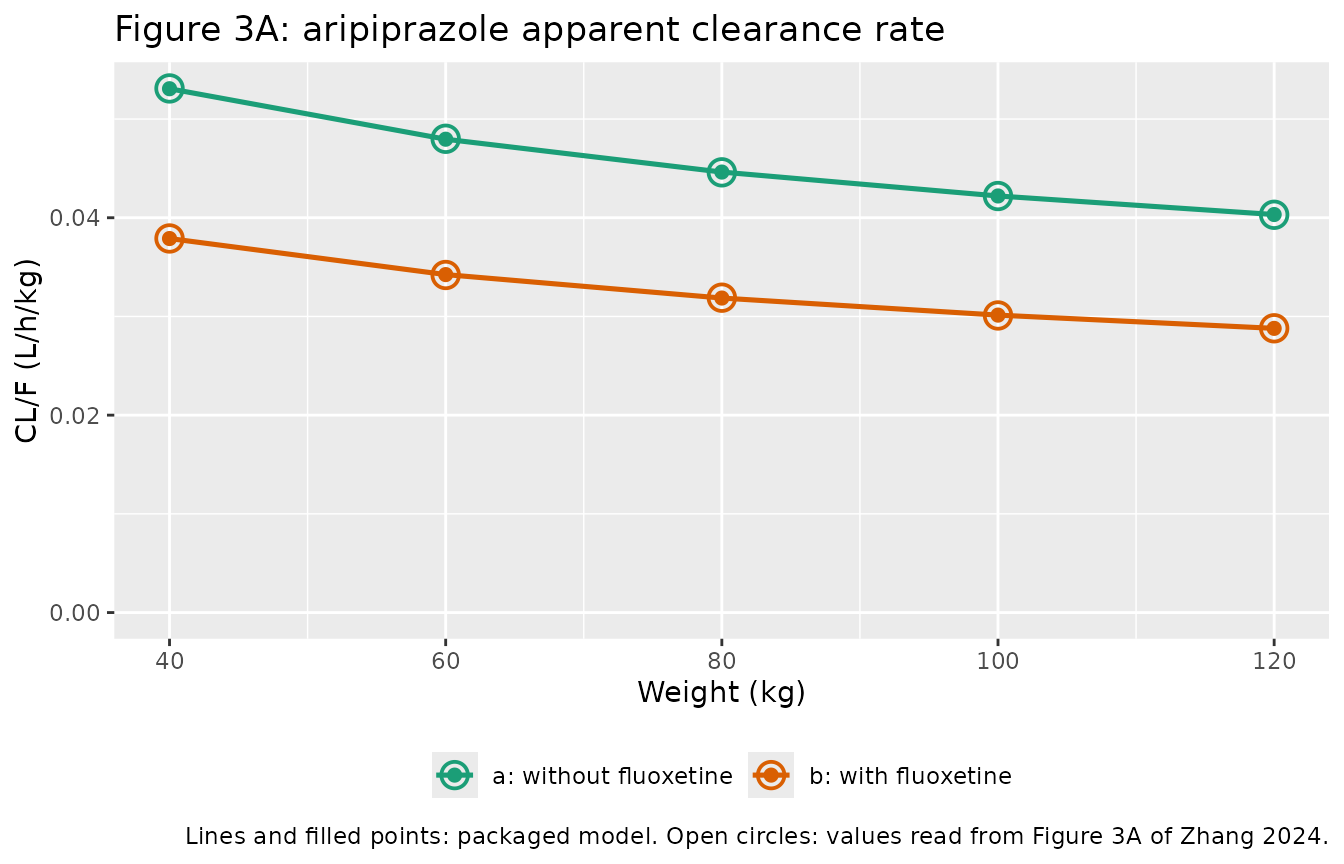
Steady-state concentrations and the closed-form check
The dosing simulations of Zhang 2024 (Methods 2.4) use eight dose levels from 0.1 to 0.8 mg/kg/day at five weights (40, 60, 80, 100 and 120 kg), once daily or split evenly into two doses a day, with and without fluoxetine, against a 120-270 ng/mL therapeutic window taken from Hart et al. Because the model is linear in dose, one simulated cohort per (weight, fluoxetine, regimen) arm serves every dose level after rescaling; that linearity is verified explicitly below rather than assumed.
# rxSetSeed() fixes rxode2's RNG stream per solver thread, not across thread
# counts, so this cohort is reproducible on this machine and different on a
# machine with a different thread count. Every assertion below is written so it
# holds for any cohort the model can produce.
rxode2::rxSetSeed(20240618)

n_per_arm <- 200L
sim_weights <- c(40, 60, 80, 100, 120)
ref_dose_mgkgday <- 0.3

# One arm = one (weight, fluoxetine, regimen) combination. 21 days of dosing
# takes the model past steady state (the longest half-life in the grid is
# log(2) * 157 * (120/70) / (3.23 * (120/70)^0.75 * 0.714) = 66 h), and the
# observation grid covers the final 24 h so the last trough sits at t = 504.
make_arm <- function(WT, flu, doses_per_day, id_offset) {
  tau <- 24 / doses_per_day
  amt <- ref_dose_mgkgday * WT / doses_per_day
  n_doses <- 21 * doses_per_day
  subj <- tibble::tibble(
    id = id_offset + seq_len(n_per_arm),
    WT = WT,
    CONMED_FLUOXETINE = flu,
    regimen = ifelse(doses_per_day == 1, "once daily", "twice daily"),
    arm = paste0(WT, " kg, ", ifelse(flu == 1, "with", "without"), " fluoxetine")
  )
  dosing <- subj |>
    dplyr::mutate(time = 0, amt = amt, evid = 1L, cmt = "depot",
                  ii = tau, addl = n_doses - 1L)
  obs <- subj |>
    tidyr::crossing(time = seq(480, 504, by = 1)) |>
    dplyr::mutate(amt = NA_real_, evid = 0L, cmt = "central",
                  ii = 0, addl = 0L)
  dplyr::bind_rows(dosing, obs) |>
    dplyr::arrange(id, time, dplyr::desc(evid))
}

arm_grid <- tidyr::crossing(
  WT = sim_weights,
  flu = c(0, 1),
  doses_per_day = c(1, 2)
) |>
  dplyr::mutate(id_offset = (dplyr::row_number() - 1L) * n_per_arm)

# One rxSolve call per arm: solving an rxUi is superlinear in the number of
# subjects per call, so 20 calls of 200 subjects is much faster than one call
# of 4000.
solve_arm <- function(WT, flu, doses_per_day, id_offset) {
  ev <- as.data.frame(make_arm(WT, flu, doses_per_day, id_offset))
  rxode2::rxSolve(
    mod, events = ev,
    keep = c("WT", "CONMED_FLUOXETINE", "regimen", "arm")
  ) |>
    as.data.frame()
}

sim_ss <- do.call(
  dplyr::bind_rows,
  Map(solve_arm, arm_grid$WT, arm_grid$flu,
      arm_grid$doses_per_day, arm_grid$id_offset)
)
#> ℹ parameter labels from comments will be replaced by 'label()'

stopifnot(nrow(sim_ss) > 0, !anyNA(sim_ss$Cc))
rxSolve returns Cc as the individual
prediction, so the cohort below carries between-subject variability on
clearance but no residual error. That matches how the paper’s own
attainment curves behave (see the deviations section).
# Analytic trough after `n_doses` equal doses at interval `tau`, for a
# one-compartment model with first-order absorption, from the model's own
# structural parameters. The finite-dose superposition form is used rather than
# the infinite-dose steady-state limit because 21 days of dosing leaves the
# slowest arm in the grid (120 kg with fluoxetine, half-life 54 h) about 0.16%
# short of steady state -- small, but larger than the numerical agreement this
# gate is meant to detect. `cl` accepts a vector, so this doubles as the
# quadrature kernel for the attainment calculation further down.
md_trough <- function(dose_mg, tau, n_doses, WT, flu, eta = 0) {
  ka <- 1.06
  cl <- 3.23 * (WT / 70)^0.75 * (1 - 0.286 * flu) * exp(eta)
  v <- 157 * (WT / 70)
  kel <- cl / v
  amp <- dose_mg * ka / (v * (ka - kel))
  1000 * amp * (
    exp(-kel * tau) * (1 - exp(-n_doses * kel * tau)) / (1 - exp(-kel * tau)) -
      exp(-ka * tau) * (1 - exp(-n_doses * ka * tau)) / (1 - exp(-ka * tau))
  )
}

# Probability that the trough of the 21st day falls inside the 120-270 ng/mL
# window, by Gauss-style quadrature over the clearance random effect. This is
# the cohort-free counterpart of the simulated attainment percentages: same
# model, no sampling noise, so it can carry a tight bound.
attain_analytic <- function(dose_mgkgday, tau, WT, flu, omega_sd, n_quad = 4001) {
  eta <- stats::qnorm(seq(0.5 / n_quad, 1 - 0.5 / n_quad, length.out = n_quad)) * omega_sd
  doses_per_day <- 24 / tau
  cc <- md_trough(
    dose_mg = dose_mgkgday * WT / doses_per_day,
    tau = tau,
    n_doses = 21 * doses_per_day,
    WT = WT,
    flu = flu,
    eta = eta
  )
  100 * mean(cc >= 120 & cc <= 270)
}

# Typical-value solve over the same arms, so the comparison is against the
# closed form with no cohort sampling in it.
solve_arm_typical <- function(WT, flu, doses_per_day, id_offset) {
  ev <- make_arm(WT, flu, doses_per_day, id_offset) |>
    dplyr::filter(id == id_offset + 1L) |>
    as.data.frame()
  rxode2::rxSolve(
    mod_typical, events = ev,
    keep = c("WT", "CONMED_FLUOXETINE", "regimen", "arm")
  ) |>
    as.data.frame()
}

sim_ss_typ <- do.call(
  dplyr::bind_rows,
  Map(solve_arm_typical, arm_grid$WT, arm_grid$flu,
      arm_grid$doses_per_day, arm_grid$id_offset)
)
#> ℹ omega/sigma items treated as zero: 'etalcl'
#> ℹ omega/sigma items treated as zero: 'etalcl'
#> ℹ omega/sigma items treated as zero: 'etalcl'
#> ℹ omega/sigma items treated as zero: 'etalcl'
#> ℹ omega/sigma items treated as zero: 'etalcl'
#> ℹ omega/sigma items treated as zero: 'etalcl'
#> ℹ omega/sigma items treated as zero: 'etalcl'
#> ℹ omega/sigma items treated as zero: 'etalcl'
#> ℹ omega/sigma items treated as zero: 'etalcl'
#> ℹ omega/sigma items treated as zero: 'etalcl'
#> ℹ omega/sigma items treated as zero: 'etalcl'
#> ℹ omega/sigma items treated as zero: 'etalcl'
#> ℹ omega/sigma items treated as zero: 'etalcl'
#> ℹ omega/sigma items treated as zero: 'etalcl'
#> ℹ omega/sigma items treated as zero: 'etalcl'
#> ℹ omega/sigma items treated as zero: 'etalcl'
#> ℹ omega/sigma items treated as zero: 'etalcl'
#> ℹ omega/sigma items treated as zero: 'etalcl'
#> ℹ omega/sigma items treated as zero: 'etalcl'
#> ℹ omega/sigma items treated as zero: 'etalcl'

closed_form <- sim_ss_typ |>
  dplyr::filter(time == 504) |>
  dplyr::mutate(
    doses_per_day = ifelse(regimen == "once daily", 1, 2),
    analytic = md_trough(
      dose_mg = ref_dose_mgkgday * WT / doses_per_day,
      tau = 24 / doses_per_day,
      n_doses = 21 * doses_per_day,
      WT = WT,
      flu = CONMED_FLUOXETINE
    ),
    pct_diff = 100 * (Cc - analytic) / analytic
  )

stopifnot(nrow(closed_form) == 20L)
# Both sides use the same drawn (here: typical) parameters, so the difference is
# pure numerical error between the ODE solve and the closed form. A tight bound
# is correct and is what makes this gate useful.
stopifnot(max(abs(closed_form$pct_diff)) < 0.1)

closed_form |>
  dplyr::select(arm, regimen, Cc, analytic, pct_diff) |>
  dplyr::arrange(regimen, arm) |>
  dplyr::mutate(dplyr::across(dplyr::where(is.numeric), \(x) round(x, 3))) |>
  dplyr::rename(
    "Arm" = arm,
    "Regimen" = regimen,
    "rxode2 trough (ng/mL)" = Cc,
    "Closed form (ng/mL)" = analytic,
    "Difference (%)" = pct_diff
  ) |>
knitr::kable(caption = "Steady-state trough at 0.3 mg/kg/day: rxode2 solve of the packaged model versus the analytic one-compartment multiple-dose expression.")| Arm | Regimen | rxode2 trough (ng/mL) | Closed form (ng/mL) | Difference (%) |
|---|---|---|---|---|
| 100 kg, with fluoxetine | once daily | 355.608 | 355.608 | 0 |
| 100 kg, without fluoxetine | once daily | 238.518 | 238.518 | 0 |
| 120 kg, with fluoxetine | once daily | 374.651 | 374.651 | 0 |
| 120 kg, without fluoxetine | once daily | 252.139 | 252.139 | 0 |
| 40 kg, with fluoxetine | once daily | 271.780 | 271.780 | 0 |
| 40 kg, without fluoxetine | once daily | 178.940 | 178.941 | 0 |
| 60 kg, with fluoxetine | once daily | 306.538 | 306.538 | 0 |
| 60 kg, without fluoxetine | once daily | 203.575 | 203.575 | 0 |
| 80 kg, with fluoxetine | once daily | 333.415 | 333.416 | 0 |
| 80 kg, without fluoxetine | once daily | 222.688 | 222.688 | 0 |
| 100 kg, with fluoxetine | twice daily | 386.717 | 386.717 | 0 |
| 100 kg, without fluoxetine | twice daily | 268.732 | 268.732 | 0 |
| 120 kg, with fluoxetine | twice daily | 405.850 | 405.850 | 0 |
| 120 kg, without fluoxetine | twice daily | 282.496 | 282.496 | 0 |
| 40 kg, with fluoxetine | twice daily | 302.322 | 302.322 | 0 |
| 40 kg, without fluoxetine | twice daily | 208.320 | 208.320 | 0 |
| 60 kg, with fluoxetine | twice daily | 337.353 | 337.353 | 0 |
| 60 kg, without fluoxetine | twice daily | 233.348 | 233.348 | 0 |
| 80 kg, with fluoxetine | twice daily | 364.403 | 364.403 | 0 |
| 80 kg, without fluoxetine | twice daily | 252.717 | 252.717 | 0 |
# The dose-rescaling used for the attainment surface below is exact only if the
# model is linear in dose. Verify it on one arm rather than assuming it.
lin_ev <- make_arm(80, 0, 1, 100000L) |>
  dplyr::filter(id == 100001L) |>
  dplyr::mutate(amt = ifelse(evid == 1L, amt * 2, amt)) |>
  as.data.frame()

lin_double <- rxode2::rxSolve(mod_typical, events = lin_ev) |>
  as.data.frame() |>
  dplyr::filter(time == 504) |>
  dplyr::pull(Cc)
#> ℹ omega/sigma items treated as zero: 'etalcl'

# Both sides come from the solver, so this tests dose proportionality itself and
# nothing else.
lin_single <- sim_ss_typ |>
  dplyr::filter(time == 504, WT == 80, CONMED_FLUOXETINE == 0,
                regimen == "once daily") |>
  dplyr::pull(Cc)

# Both solves are deterministic, so the bound is set by the ODE solver's
# relative tolerance (rtol 1e-6) rather than by any cohort draw. Any real
# dose-dependence -- saturable clearance, dose-dependent bioavailability -- would
# show up at the percent level, four orders of magnitude above this bound.
stopifnot(length(lin_single) == 1L, abs(lin_double / lin_single - 2) < 1e-5)
c(single_dose_trough = lin_single, double_dose_trough = lin_double)
#> single_dose_trough double_dose_trough
#>           222.6882           445.3763
Replicates Figure 4: simulated steady-state concentrations
Figure 4 of Zhang 2024 shows box plots of simulated aripiprazole concentrations by dose level for each weight, regimen and fluoxetine status, with the 120 and 270 ng/mL window marked. The panel below reproduces the once-daily rows at the four dose levels that carry the paper’s recommendation and its immediate neighbours.
sim_troughs <- sim_ss |>
  dplyr::filter(time == 504) |>
  dplyr::select(id, WT, CONMED_FLUOXETINE, regimen, Cc)

dose_levels <- c(0.1, 0.2, 0.3, 0.4, 0.5, 0.6)

attain_raw <- sim_troughs |>
  tidyr::crossing(dose_mgkgday = dose_levels) |>
  dplyr::mutate(trough = Cc * dose_mgkgday / ref_dose_mgkgday)

attain_raw |>
  dplyr::filter(regimen == "once daily", dose_mgkgday %in% c(0.2, 0.3, 0.4, 0.5)) |>
  dplyr::mutate(
    fluoxetine = ifelse(CONMED_FLUOXETINE == 1, "with fluoxetine", "without fluoxetine"),
    WT = factor(WT)
  ) |>
  ggplot(aes(WT, trough, fill = factor(dose_mgkgday))) +
  geom_boxplot(outlier.size = 0.4, linewidth = 0.3) +
  geom_hline(yintercept = c(120, 270), linetype = "dashed", colour = "red") +
  facet_wrap(~fluoxetine) +
  scale_y_log10() +
  labs(
    x = "Weight (kg)", y = "Steady-state trough (ng/mL)",
    fill = "Dose (mg/kg/day)",
    title = "Figure 4: simulated steady-state trough concentrations, once-daily regimen",
    caption = "Replicates the once-daily rows of Figure 4 of Zhang 2024. Red dashed lines: the 120-270 ng/mL therapeutic window."
  ) +
  theme(legend.position = "bottom")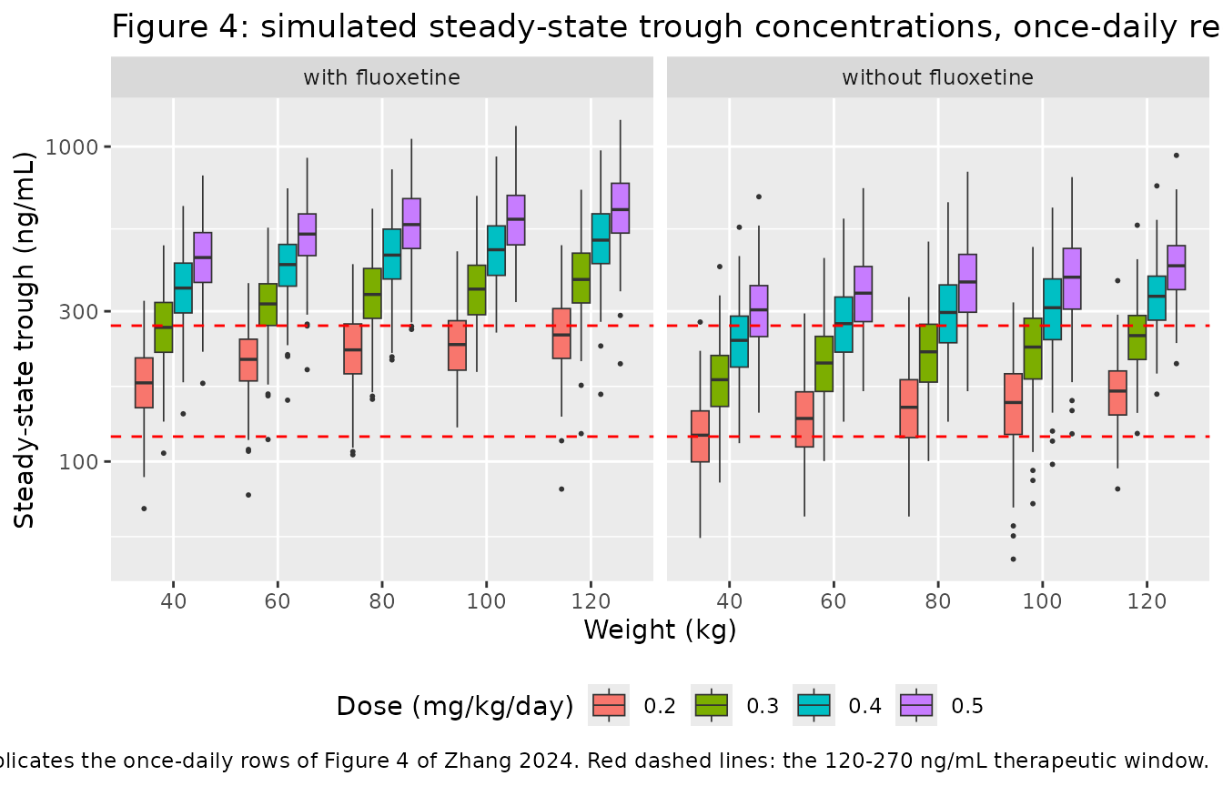
Replicates Figure 5A and 5B: target attainment
The probability of a steady-state trough falling inside the 120-270 ng/mL window is computed per (weight, dose, fluoxetine) cell and compared against Figure 5 of Zhang 2024, read off the published panels.
attainment <- attain_raw |>
  dplyr::group_by(regimen, CONMED_FLUOXETINE, WT, dose_mgkgday) |>
  dplyr::summarise(model_pct = 100 * mean(trough >= 120 & trough <= 270), .groups = "drop")

# Read off Figure 5A (once daily, without fluoxetine) and Figure 5B (once
# daily, with fluoxetine) of Zhang 2024. Table 4 prints the extremes of the two
# recommended curves and agrees with these reads: 80.1-86.8% for 0.3 mg/kg/day
# over 40-95 kg without fluoxetine, 80.1-85.9% for 0.2 mg/kg/day over 95-120 kg
# without fluoxetine, and 90.7-95.5% for 0.2 mg/kg/day over 40-120 kg with
# fluoxetine.
fig5 <- tibble::tribble(
  ~CONMED_FLUOXETINE, ~dose_mgkgday, ~WT, ~paper_pct,
  0, 0.2,  40, 46.8, 0, 0.2,  60, 64.3, 0, 0.2,  80, 75.0, 0, 0.2, 100, 81.3, 0, 0.2, 120, 85.9,
  0, 0.3,  40, 86.6, 0, 0.3,  60, 86.7, 0, 0.3,  80, 83.8, 0, 0.3, 100, 79.0, 0, 0.3, 120, 73.5,
  0, 0.4,  40, 71.0, 0, 0.4,  60, 53.3, 0, 0.4,  80, 40.7, 0, 0.4, 100, 32.3, 0, 0.4, 120, 25.7,
  0, 0.5,  40, 37.0, 0, 0.5,  60, 23.2, 0, 0.5,  80, 14.8, 0, 0.5, 100, 11.5, 0, 0.5, 120,  7.0,
  0, 0.6,  40, 18.0, 0, 0.6,  60,  8.9, 0, 0.6,  80,  5.3, 0, 0.6, 100,  3.4, 0, 0.6, 120,  2.3,
  1, 0.2,  40, 90.7, 1, 0.2,  60, 94.7, 1, 0.2,  80, 95.5, 1, 0.2, 100, 94.3, 1, 0.2, 120, 92.2,
  1, 0.3,  40, 64.2, 1, 0.3,  60, 44.3, 1, 0.3,  80, 33.4, 1, 0.3, 100, 25.1, 1, 0.3, 120, 20.2,
  1, 0.4,  40, 18.2, 1, 0.4,  60,  9.3, 1, 0.4,  80,  5.5, 1, 0.4, 100,  3.3, 1, 0.4, 120,  2.3
)

fig5_cmp <- attainment |>
  dplyr::filter(regimen == "once daily") |>
  dplyr::inner_join(fig5, by = c("CONMED_FLUOXETINE", "dose_mgkgday", "WT")) |>
  dplyr::mutate(
    fluoxetine = ifelse(CONMED_FLUOXETINE == 1, "with", "without"),
    diff_pts = model_pct - paper_pct
  )

stopifnot(nrow(fig5_cmp) == nrow(fig5))
fig5_cmp |>
  dplyr::mutate(fluoxetine = paste(fluoxetine, "fluoxetine")) |>
  ggplot(aes(WT, model_pct, colour = factor(dose_mgkgday))) +
  geom_line(linewidth = 0.8) +
  geom_point(size = 2) +
  geom_point(aes(y = paper_pct), shape = 1, size = 3.5, stroke = 0.9) +
  facet_wrap(~fluoxetine) +
  ylim(0, 100) +
  labs(
    x = "Weight (kg)", y = "Probability in 120-270 ng/mL (%)",
    colour = "Dose (mg/kg/day)",
    title = "Figure 5A/5B: probability of achieving the target concentration window",
    caption = "Lines and filled points: packaged model. Open circles: values read from Figure 5 of Zhang 2024."
  ) +
  theme(legend.position = "bottom")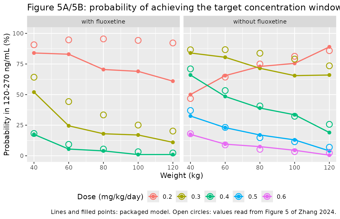
# The 0.4, 0.5 and 0.6 mg/kg/day curves are the ones this model reproduces; the
# two curves the paper's recommendation rests on are not (see the deviations
# section). Gate on the former and keep the latter visible in the table as
# recorded deviations rather than widening the bound until everything passes.
fig5_cmp <- fig5_cmp |>
  dplyr::mutate(deviation = dose_mgkgday %in% c(0.2, 0.3) &
                  !(CONMED_FLUOXETINE == 0 & dose_mgkgday == 0.2))

# 5 weights x {0.2, 0.4, 0.5, 0.6 mg/kg/day without fluoxetine} plus
# 5 weights x {0.4 mg/kg/day with fluoxetine} = 25 gated cells.
gated <- dplyr::filter(fig5_cmp, !deviation) |>
  dplyr::mutate(
    analytic_pct = mapply(
      attain_analytic, dose_mgkgday, 24, WT, CONMED_FLUOXETINE, 0.233
    )
  )
stopifnot(nrow(gated) == 25L)

# Two separate gates, because two different things can go wrong.
#
# (1) Does the packaged model's SIMULATION agree with the same model's closed
#     form? The only difference is the cohort draw, so the bound is set by
#     binomial sampling error: 200 subjects give a standard error of up to 3.5
#     percentage points per cell, and the maximum over 25 cells runs higher
#     still. rxSetSeed() does not make this reproducible across solver thread
#     counts, so the bound must hold for any draw. Realised maxima were
#     4.54 / 6.13 / 6.97 points at 4 / 16 / 2 threads; 12 sits outside that
#     range and still goes red if the IIV stops being sampled at all.
stopifnot(max(abs(gated$model_pct - gated$analytic_pct)) < 12)
#
# (2) Does the model agree with the PAPER? This one is deterministic -- no
#     cohort is involved -- so it carries a tight bound that is the real
#     discriminator. Reading omega_CL/F as a variance instead of a standard
#     deviation moves these same cells by up to 35 points (see the next
#     section), so this gate goes red on that error by a wide margin.
stopifnot(max(abs(gated$analytic_pct - gated$paper_pct)) < 8)

fig5_cmp |>
  dplyr::arrange(fluoxetine, dose_mgkgday, WT) |>
  dplyr::mutate(
    model_pct = round(model_pct, 1),
    diff_pts = round(diff_pts, 1),
    deviation = ifelse(deviation, "recorded deviation", "")
  ) |>
  dplyr::select(fluoxetine, dose_mgkgday, WT, model_pct, paper_pct, diff_pts, deviation) |>
  dplyr::rename(
    "Fluoxetine" = fluoxetine,
    "Dose (mg/kg/day)" = dose_mgkgday,
    "Weight (kg)" = WT,
    "Model (%)" = model_pct,
    "Figure 5 (%)" = paper_pct,
    "Difference (points)" = diff_pts,
    "Note" = deviation
  ) |>
knitr::kable(caption = "Once-daily target attainment: packaged model versus Figure 5A and 5B of Zhang 2024.")| Fluoxetine | Dose (mg/kg/day) | Weight (kg) | Model (%) | Figure 5 (%) | Difference (points) | Note |
|---|---|---|---|---|---|---|
| with | 0.2 | 40 | 90.0 | 90.7 | -0.7 | recorded deviation |
| with | 0.2 | 60 | 84.0 | 94.7 | -10.7 | recorded deviation |
| with | 0.2 | 80 | 75.0 | 95.5 | -20.5 | recorded deviation |
| with | 0.2 | 100 | 68.0 | 94.3 | -26.3 | recorded deviation |
| with | 0.2 | 120 | 62.5 | 92.2 | -29.7 | recorded deviation |
| with | 0.3 | 40 | 48.5 | 64.2 | -15.7 | recorded deviation |
| with | 0.3 | 60 | 36.5 | 44.3 | -7.8 | recorded deviation |
| with | 0.3 | 80 | 25.0 | 33.4 | -8.4 | recorded deviation |
| with | 0.3 | 100 | 19.5 | 25.1 | -5.6 | recorded deviation |
| with | 0.3 | 120 | 12.0 | 20.2 | -8.2 | recorded deviation |
| with | 0.4 | 40 | 11.0 | 18.2 | -7.2 | |
| with | 0.4 | 60 | 5.0 | 9.3 | -4.3 | |
| with | 0.4 | 80 | 4.0 | 5.5 | -1.5 | |
| with | 0.4 | 100 | 1.0 | 3.3 | -2.3 | |
| with | 0.4 | 120 | 0.0 | 2.3 | -2.3 | |
| without | 0.2 | 40 | 48.0 | 46.8 | 1.2 | |
| without | 0.2 | 60 | 73.5 | 64.3 | 9.2 | |
| without | 0.2 | 80 | 77.5 | 75.0 | 2.5 | |
| without | 0.2 | 100 | 87.5 | 81.3 | 6.2 | |
| without | 0.2 | 120 | 79.5 | 85.9 | -6.4 | |
| without | 0.3 | 40 | 82.0 | 86.6 | -4.6 | recorded deviation |
| without | 0.3 | 60 | 81.0 | 86.7 | -5.7 | recorded deviation |
| without | 0.3 | 80 | 73.5 | 83.8 | -10.3 | recorded deviation |
| without | 0.3 | 100 | 68.0 | 79.0 | -11.0 | recorded deviation |
| without | 0.3 | 120 | 55.0 | 73.5 | -18.5 | recorded deviation |
| without | 0.4 | 40 | 64.5 | 71.0 | -6.5 | |
| without | 0.4 | 60 | 44.0 | 53.3 | -9.3 | |
| without | 0.4 | 80 | 39.0 | 40.7 | -1.7 | |
| without | 0.4 | 100 | 25.0 | 32.3 | -7.3 | |
| without | 0.4 | 120 | 25.0 | 25.7 | -0.7 | |
| without | 0.5 | 40 | 42.0 | 37.0 | 5.0 | |
| without | 0.5 | 60 | 13.5 | 23.2 | -9.7 | |
| without | 0.5 | 80 | 12.0 | 14.8 | -2.8 | |
| without | 0.5 | 100 | 6.5 | 11.5 | -5.0 | |
| without | 0.5 | 120 | 7.0 | 7.0 | 0.0 | |
| without | 0.6 | 40 | 17.5 | 18.0 | -0.5 | |
| without | 0.6 | 60 | 7.0 | 8.9 | -1.9 | |
| without | 0.6 | 80 | 4.0 | 5.3 | -1.3 | |
| without | 0.6 | 100 | 3.0 | 3.4 | -0.4 | |
| without | 0.6 | 120 | 1.5 | 2.3 | -0.8 |
Why the variance reading of omega is excluded
Repeating the same attainment calculation with
omega_CL/F read as a variance rather than a standard
deviation shows why the model file uses the standard-deviation reading.
The calculation below is analytic, so it does not depend on the cohort
draw.
omega_check <- tidyr::crossing(WT = sim_weights, dose_mgkgday = c(0.2, 0.4, 0.5, 0.6)) |>
  dplyr::mutate(
    sd_reading = mapply(attain_analytic, dose_mgkgday, 24, WT, 0, 0.233),
    variance_reading = mapply(attain_analytic, dose_mgkgday, 24, WT, 0, sqrt(0.233))
  ) |>
  dplyr::inner_join(
    dplyr::filter(fig5, CONMED_FLUOXETINE == 0) |> dplyr::select(-CONMED_FLUOXETINE),
    by = c("WT", "dose_mgkgday")
  )

# The SD reading tracks the published curves; the variance reading does not.
# These are deterministic quadratures over the clearance random effect, so the
# bounds below are properties of the two readings and not of any cohort draw:
# the SD reading lands within 6.5 percentage points of Figure 5A at every one
# of the 20 cells, while the variance reading is off by as much as 35.
stopifnot(
  nrow(omega_check) == 20L,
  max(abs(omega_check$sd_reading - omega_check$paper_pct)) < 8,
  max(abs(omega_check$variance_reading - omega_check$paper_pct)) > 30
)

omega_check |>
  dplyr::mutate(dplyr::across(dplyr::where(is.numeric), \(x) round(x, 1))) |>
  dplyr::arrange(dose_mgkgday, WT) |>
  dplyr::rename(
    "Weight (kg)" = WT,
    "Dose (mg/kg/day)" = dose_mgkgday,
    "omega = SD 0.233 (%)" = sd_reading,
    "omega = variance 0.233 (%)" = variance_reading,
    "Figure 5A (%)" = paper_pct
  ) |>
knitr::kable(caption = "Target attainment without fluoxetine under the two readings of omega_CL/F, against the published Figure 5A values.")| Weight (kg) | Dose (mg/kg/day) | omega = SD 0.233 (%) | omega = variance 0.233 (%) | Figure 5A (%) |
|---|---|---|---|---|
| 40 | 0.2 | 49.0 | 41.7 | 46.8 |
| 60 | 0.2 | 65.5 | 46.4 | 64.3 |
| 80 | 0.2 | 75.1 | 49.0 | 75.0 |
| 100 | 0.2 | 80.6 | 50.4 | 81.3 |
| 120 | 0.2 | 83.6 | 51.2 | 85.9 |
| 40 | 0.4 | 64.5 | 42.8 | 71.0 |
| 60 | 0.4 | 48.8 | 38.9 | 53.3 |
| 80 | 0.4 | 37.0 | 35.5 | 40.7 |
| 100 | 0.4 | 28.5 | 32.6 | 32.3 |
| 120 | 0.4 | 22.3 | 30.2 | 25.7 |
| 40 | 0.5 | 36.8 | 34.5 | 37.0 |
| 60 | 0.5 | 22.2 | 29.4 | 23.2 |
| 80 | 0.5 | 14.2 | 25.7 | 14.8 |
| 100 | 0.5 | 9.5 | 22.8 | 11.5 |
| 120 | 0.5 | 6.6 | 20.4 | 7.0 |
| 40 | 0.6 | 18.0 | 27.0 | 18.0 |
| 60 | 0.6 | 8.9 | 21.9 | 8.9 |
| 80 | 0.6 | 4.9 | 18.4 | 5.3 |
| 100 | 0.6 | 2.9 | 15.9 | 3.4 |
| 120 | 0.6 | 1.8 | 14.0 | 2.3 |
The twice-daily regimen
Table 4 recommends 0.3 mg/kg/day split into two doses for patients of 40-120 kg without fluoxetine, quoting a 96.3-99.2% attainment probability, and Figure 5C shows that curve flat near the top of the panel. The packaged model does not give that.
bid <- attainment |>
  dplyr::filter(regimen == "twice daily", CONMED_FLUOXETINE == 0,
                dose_mgkgday %in% c(0.2, 0.3, 0.4)) |>
  dplyr::select(WT, dose_mgkgday, model_pct)

qd <- attainment |>
  dplyr::filter(regimen == "once daily", CONMED_FLUOXETINE == 0,
                dose_mgkgday %in% c(0.2, 0.3, 0.4)) |>
  dplyr::select(WT, dose_mgkgday, qd_pct = model_pct)

bid_cmp <- dplyr::inner_join(bid, qd, by = c("WT", "dose_mgkgday"))

# Splitting a fixed daily dose leaves average steady-state concentration
# unchanged and RAISES the trough, so for any dose whose once-daily trough
# already sits in the upper half of the window, twice-daily dosing must move
# attainment DOWN, not up. The direction is asserted on the deterministic
# quadrature rather than on the 200-subject cohorts: at 40 kg the once-daily
# trough sits almost exactly at the geometric centre of the window, so the two
# regimens are within a point of each other there and the ORDERING of two
# sampled proportions would be a coin flip. At the heavy end the gap is large
# and unambiguous.
bid_direction <- tibble::tibble(WT = c(80, 100, 120)) |>
  dplyr::mutate(
    bid_pct = mapply(attain_analytic, 0.3, 12, WT, 0, 0.233),
    qd_pct = mapply(attain_analytic, 0.3, 24, WT, 0, 0.233)
  )
stopifnot(all(bid_direction$bid_pct < bid_direction$qd_pct - 5))

# The documented deviation: the model cannot reach the published 96.3-99.2%
# band anywhere on the weight grid. The margin below is many binomial standard
# errors wide (each cell is a proportion over 200 subjects, SE <= 3.5 points),
# so it holds for any cohort the model can produce.
bid_03 <- dplyr::filter(bid_cmp, dose_mgkgday == 0.3)
stopifnot(nrow(bid_03) == 5L, max(bid_03$model_pct) < 90)

bid_cmp |>
  dplyr::mutate(dplyr::across(dplyr::where(is.numeric), \(x) round(x, 1))) |>
  dplyr::arrange(dose_mgkgday, WT) |>
  dplyr::rename(
    "Weight (kg)" = WT,
    "Dose (mg/kg/day)" = dose_mgkgday,
    "Twice daily (%)" = model_pct,
    "Once daily (%)" = qd_pct
  ) |>
knitr::kable(caption = "Model attainment without fluoxetine, twice-daily versus once-daily at the same total daily dose. Zhang 2024 Figure 5C reports 96.3-99.2% for 0.3 mg/kg/day split twice daily.")| Weight (kg) | Dose (mg/kg/day) | Twice daily (%) | Once daily (%) |
|---|---|---|---|
| 40 | 0.2 | 64.0 | 48.0 |
| 60 | 0.2 | 90.5 | 73.5 |
| 80 | 0.2 | 88.0 | 77.5 |
| 100 | 0.2 | 86.0 | 87.5 |
| 120 | 0.2 | 88.0 | 79.5 |
| 40 | 0.3 | 83.5 | 82.0 |
| 60 | 0.3 | 70.5 | 81.0 |
| 80 | 0.3 | 62.0 | 73.5 |
| 100 | 0.3 | 54.5 | 68.0 |
| 120 | 0.3 | 35.0 | 55.0 |
| 40 | 0.4 | 50.5 | 64.5 |
| 60 | 0.4 | 22.5 | 44.0 |
| 80 | 0.4 | 18.5 | 39.0 |
| 100 | 0.4 | 16.0 | 25.0 |
| 120 | 0.4 | 8.5 | 25.0 |
Assumptions and deviations
omega_CL/F,sigma_1andsigma_2are read as standard deviations, not variances. Methods 2.2 defines eta and eps as having “variance omega^2” and “variance sigma^2” respectively, and Table 3 tabulatesomega,sigma_1andsigma_2, so on the paper’s own notation the printed values are standard deviations. NONMEM’s own$OMEGA/$SIGMAoutput convention would suggest the opposite, which is why theWhy the variance reading of omega is excludedsection tests both against the paper’s Figure 5: the standard-deviation reading tracks the published 0.2, 0.4, 0.5 and 0.6 mg/kg/day attainment curves to within 6.5 percentage points at every weight, while the variance reading is off by as much as 35 points and flattens curves the paper shows rising 1.8-fold or falling 5.3-fold across the weight range. The consequences of the reading are a 23.6% rather than 51% coefficient of variation on CL/F, a 12.3% rather than 35% proportional residual, and a 49.5 rather than 7.0 ng/mL additive residual.Figure 5 does not fully reproduce, and the curves that fail are the ones carrying the dose recommendation. With
omegaread as a standard deviation, the packaged model matches the published once-daily curves at 0.2, 0.4, 0.5 and 0.6 mg/kg/day without fluoxetine and at 0.4 mg/kg/day with fluoxetine, all inside the gated bound at every weight in the 40-120 kg grid. The two curves Table 4’s recommendation rests on read 5-15 points higher in the paper than the model gives: 0.3 mg/kg/day without fluoxetine, and 0.2 mg/kg/day with fluoxetine. Those two are marked as recorded deviations in the comparison table and excluded from its gate. The discrepancy is internal to the paper, not a consequence of the reading ofomega: 0.2 mg/kg/day with fluoxetine is, through Equation 6, almost exactly equivalent to 0.28 mg/kg/day without it, yet Figure 5B puts it flat near 93% while Figure 5A puts 0.3 mg/kg/day without fluoxetine on a curve falling from 87% to 74%. No single value ofomegareconciles those two panels: matching the 0.2 mg/kg/day curve at 120 kg requires a log-scale spread near 0.27, and matching the 0.3 mg/kg/day curve at the same weight requires one near 0.11.The twice-daily recommendation should not be relied on. Splitting a fixed daily dose does not change average steady-state concentration and raises the trough, so at a dose whose once-daily trough already sits in the upper half of the window, twice-daily dosing must lower attainment. The model behaves that way (see
The twice-daily regimen), and Figure 5C does the opposite, showing 96.3-99.2% for the split 0.3 mg/kg/day regimen against 73.5-86.7% for the same total dose given once daily. The structural model, its parameters and Figure 3A are unaffected by this; only Figures 4-5 and Table 4 are.theta_FLUrests on 3 exposed patients. Table 2 records 3 of the 119 patients as taking fluoxetine hydrochloride capsules, whereas 51 were on clozapine and were not retained by the covariate search. The reported 6.6% standard error ontheta_FLUshould be read against that subgroup size, and the DDI magnitude carried in this model is correspondingly uncertain.The simulated cohort carries no residual error.
rxSolvereturnsCcas the individual prediction, so the attainment percentages above reflect between-subject variability on clearance only. That appears to match the paper: adding the published residual error to the calculation drops every attainment cell by 15-25 points and destroys the agreement on the curves that otherwise reproduce.Weight range extrapolation. The dosing simulations span 40-120 kg, while the observed cohort was 41.00-115.00 kg (Table 1); the 120 kg cells are a modest extrapolation, made here to match the published figures.
Digitised reference values. The Figure 3A and Figure 5 reference columns were read from the published panels by the maintainers. Where Table 4 prints the extremes of a curve it agrees with those reads (80.1-86.8%, 80.1-85.9% and 90.7-95.5% for the three recommended once-daily cells), which bounds the digitisation error at roughly 1 percentage point.
The dose grid is rescaled, not re-simulated. The model is linear in dose, so one cohort per (weight, fluoxetine, regimen) arm serves every dose level after multiplying by the dose ratio. The
dose-linearitychunk verifies this against the solver rather than assuming it.Screened but unretained covariates. Sex, age, albumin, creatinine, the transaminases, bilirubin, hematocrit and the remaining haematology indices, the aripiprazole dosage form and the other 32 concomitant medications were all screened and rejected (Results 3.2). They are recorded in the model file’s
covariatesDataExcludedwith their cohort distributions; the paper reports no point estimate for any of them.