Meropenem and C-reactive protein (Troisi 2024)
Source:vignettes/articles/Troisi_2024_meropenem.Rmd
Troisi_2024_meropenem.RmdModel and source
- Citation: Troisi C, Cojutti PG, Rinaldi M, Tonetti T, Siniscalchi A, van Hasselt C, Viale P, Pea F. Impact of Continuous Infusion Meropenem PK/PD Target Attainment on C-Reactive Protein Dynamics in Critically Ill Patients With Documented Gram-Negative Hospital-Acquired or Ventilator-Associated Pneumonia. Clin Pharmacokinet. 2024;63(11):1573-1583. doi:10.1007/s40262-024-01436-6
- Description: Sequential population PK/PD model of continuous-infusion meropenem and plasma C-reactive protein (C-RP) in critically ill adults with documented Gram-negative hospital-acquired or ventilator-associated pneumonia. One-compartment intravenous PK with the volume fixed at 20 L and clearance rising exponentially (uncentered) with CKD-EPI eGFR. Meropenem concentration inhibits C-RP production in an indirect-response (turnover) model with FULL inhibition (Imax = 1); the C-RP baseline R0 is estimated and kin = R0 * kout. The IC50 rises exponentially (uncentered) with the meropenem MIC of the subject’s isolate and with empirical anti-MRSA co-therapy.
- Article (open access): https://doi.org/10.1007/s40262-024-01436-6
Troisi 2024 fitted continuous-infusion (CI) meropenem plasma
concentrations and C-reactive protein (C-RP) concentrations in a
two-step sequential analysis in Monolix: a
one-compartment PK model was estimated first, and its parameters were
then held fixed while an indirect-response (turnover) model with full
inhibition of C-RP production was fitted. The published final model is
one coupled PK/PD system, so it is packaged as a single .R
file with both outputs.
Three features of the encoding are worth flagging before the numbers:
- Both covariate relationships are uncentered
exponentials.
CL = 2.72 x e^(0.011 x eGFR)(Results), soexp(lcl) = 2.72 L/his the clearance extrapolated to eGFR = 0; andIC50 = 0.79 x e^(0.44 x MIC) x e^(2.46 x DRUG), soexp(lic50) = 0.79 mg/Lis the IC50 at MIC = 0 without anti-MRSA co-therapy. - Unlike the same group’s dalbavancin model
(
Cojutti_2024_dalbavancin), the C-RP baseline is estimated (C-RP0 = 22.58 mg/dL, Table 3) and is not supplied as data. - The volume is fixed at 20 L from the group’s
earlier meropenem model (
Cojutti_2021_meropenem), because a continuous infusion carries no information on V.
Population
Sixty-four critically ill adults with documented Gram-negative hospital-acquired (HAP) or ventilator-associated pneumonia (VAP), treated with CI meropenem under real-time therapeutic drug monitoring at a single Italian centre between December 2020 and August 2023 (Patients and Methods). Median (IQR) age 65.5 (57.0-74.0) years, weight 75.0 (65.0-85.0) kg, 28/64 (43.75%) female, CKD-EPI eGFR 70.0 (39.0-100.0) mL/min/1.73 m^2; median daily dose 2 g (1.5-4) and median meropenem Css 15.9 (9.8-27.6) mg/L (Table 1). The PK model used all 64 patients (211 concentrations). The PD model used only the 47 patients on meropenem monotherapy (Fig. 2 Group A, n = 24) or meropenem plus an empirical anti-MRSA agent (Group B, n = 23), providing 328 C-RP concentrations; median observed baseline C-RP was 15.7 (9.2-26.1) mg/dL. Isolates in the PD cohort were mostly Pseudomonas aeruginosa (13), Klebsiella pneumoniae (13) and Acinetobacter baumannii (7), with a median meropenem MIC of 0.25 mg/L (IQR 0.12-4.00, range 0.12-64; Table 2).
The same information is available programmatically via
rxode2::rxode(readModelDb("Troisi_2024_meropenem"))$population.
Source trace
The per-parameter origin is recorded as an in-file comment next to
each ini() entry in
inst/modeldb/specificDrugs/Troisi_2024_meropenem.R. The
table below collects them in one place.
| Equation / parameter | Value | Source location |
|---|---|---|
lcl (CL intercept at eGFR = 0) |
2.72 L/h | Table 3, ‘CLMER’; Results equation
CL (L/h) = 2.72 x e^(0.011 x eGFR)
|
e_crcl_cl |
0.011 per mL/min/1.73 m^2 | Table 3, ‘CLCR on CLMER’; same Results equation; ESM covariate equation 1 |
lvc |
20 L (fixed) | Table 3, ‘V (L) 20 (fixed)’; Methods (‘V was fixed at 20 L, based on a previous model [16]’) |
lrbase (C-RP0) |
22.58 mg/dL | Table 3 |
lic50 |
0.79 mg/L | Table 3; Results IC50 equation |
lkout |
0.012 1/h | Table 3 |
e_mic_ic50 |
0.44 per mg/L | Table 3, ‘MIC on IC50’; ESM covariate equation 2 |
e_conmed_antimrsa_ic50 |
2.46 | Table 3, ‘Group on IC50’; ESM covariate equation 2
(DRUG) |
etalcl, etalrbase, etalic50,
etalkout
|
SD 0.59, 0.51, 1.59, 1.08 (squared into variances) | Table 3; footnote ‘omega standard deviation of inter-individual variability’ |
propSd, propSd_crp
|
0.37, 0.35 | Table 3, ‘Proportional error’ (PK and PD); footnote
observation = prediction x (1 + proportional error)
|
| One-compartment IV model, first-order elimination | n/a | Methods; ESM (‘central compartment (volume V) and a linear elimination’) |
d/dt(crp) <- kin * (1 - Cc / (Cc + ic50)) - kout * crp |
n/a | Methods equation; ESM
ddt_R = kin * (1 - Cc/(Cc+IC50)) - kout * R
|
kin <- rbase * kout,
crp(0) <- rbase
|
n/a | Methods (kin = CRP0 x kout); ESM
(R_0 = R0, kin = R0 * kout) |
Typical-value checks against the paper’s own numbers
The Discussion quotes the model’s clearance at two eGFR values. These
are a closed-form identity of the transcribed lcl and
e_crcl_cl.
mod <- readModelDb("Troisi_2024_meropenem")
ui <- rxode2::rxode(mod)
#> ℹ parameter labels from comments will be replaced by 'label()'
th <- ui$theta

cl_check <- tibble(
  eGFR = c(49, 91.5),
  `CL paper (L/h)` = c(4.66, 7.44),
  `CL model (L/h)` = exp(th[["lcl"]]) * exp(th[["e_crcl_cl"]] * eGFR)
) |>
  mutate(`Difference (%)` = 100 * (`CL model (L/h)` / `CL paper (L/h)` - 1))
knitr::kable(cl_check, digits = 2,
caption = "Typical clearance versus the Discussion of Troisi 2024.")| eGFR | CL paper (L/h) | CL model (L/h) | Difference (%) |
|---|---|---|---|
| 49.0 | 4.66 | 4.66 | 0.06 |
| 91.5 | 7.44 | 7.44 | 0.03 |
# Both values are printed to 2 decimals; a transcription slip in either
# coefficient moves CL by far more than rounding.
stopifnot(all(abs(cl_check$`Difference (%)`) < 0.5))
At steady state of a constant-rate infusion the typical model must
give Css = rate / CL, and with a constant concentration the
C-RP state approaches R0 * (1 - Css / (Css + IC50)). Both
are checked against a typical-value solve (no random effects) for a 2
g/day infusion at eGFR 70 and MIC 0.25 mg/L.
mod_typ <- rxode2::zeroRe(mod)
#> ℹ parameter labels from comments will be replaced by 'label()'
rate_typ <- 2000 / 24
ev_typ <- rxode2::et(amt = 2000 * 30, rate = rate_typ, cmt = "central") |>
  rxode2::et(seq(0, 30 * 24, by = 24), cmt = "crp")
typ_cov <- data.frame(CRCL = 70, MIC = 0.25, CONMED_ANTIMRSA = c(0, 1))
sim_typ <- lapply(seq_len(nrow(typ_cov)), function(i) {
  s <- rxode2::rxSolve(mod_typ, ev_typ, params = typ_cov[i, ], returnType = "data.frame")
  s$CONMED_ANTIMRSA <- typ_cov$CONMED_ANTIMRSA[i]
  s
}) |> bind_rows()
#> ℹ omega/sigma items treated as zero: 'etalcl', 'etalrbase', 'etalic50', 'etalkout'
#> ℹ omega/sigma items treated as zero: 'etalcl', 'etalrbase', 'etalic50', 'etalkout'

cl_typ <- exp(th[["lcl"]] + th[["e_crcl_cl"]] * 70)
css_typ <- rate_typ / cl_typ
ic50_typ <- exp(th[["lic50"]] + th[["e_mic_ic50"]] * 0.25 +
                  th[["e_conmed_antimrsa_ic50"]] * typ_cov$CONMED_ANTIMRSA)
crp_ss <- exp(th[["lrbase"]]) * (1 - css_typ / (css_typ + ic50_typ))
end_typ <- sim_typ |> filter(time == max(time))

ss_tab <- tibble(
  `Anti-MRSA co-therapy` = typ_cov$CONMED_ANTIMRSA,
  `Css closed form (mg/L)` = css_typ,
  `Css solved, day 30 (mg/L)` = end_typ$Cc,
  `C-RP closed form (mg/dL)` = crp_ss,
  `C-RP solved, day 30 (mg/dL)` = end_typ$crp
)
knitr::kable(ss_tab, digits = 3,
caption = "Typical steady state: solver versus closed form (2 g/day, eGFR 70, MIC 0.25 mg/L).")| Anti-MRSA co-therapy | Css closed form (mg/L) | Css solved, day 30 (mg/L) | C-RP closed form (mg/dL) | C-RP solved, day 30 (mg/dL) |
|---|---|---|---|---|
| 0 | 14.185 | 14.185 | 1.322 | 1.325 |
| 1 | 14.185 | 14.185 | 9.510 | 9.513 |
# Same parameters on both sides, so only numerical error separates them; the
# C-RP state is still 0.018% short of equilibrium at day 30 (exp(-0.012 * 720)).
stopifnot(all(abs(end_typ$Cc / css_typ - 1) < 1e-3))
stopifnot(all(abs(end_typ$crp / crp_ss - 1) < 1e-2))
The typical 2 g/day Css of 14.2 mg/L at the cohort median eGFR of 70 mL/min/1.73 m^2 sits close to the observed Table 1 median Css of 15.9 mg/L (the observed figure pools every dose and renal function).
Virtual cohort
Original observed data are not publicly available. The cohort follows the Monte Carlo design of Troisi 2024 Methods: five CI meropenem dosages (125 mg q8h, 500 mg q8h, 500 mg q6h, 1000 mg q6h and 1500 mg q6h, i.e. 375, 1500, 2000, 4000 and 6000 mg/day) crossed with five renal-function classes (eGFR 0-30, 31-60, 61-90, 91-120 and 121-150 mL/min/1.73 m^2), simulated separately for monotherapy and for empirical anti-MRSA co-therapy. Each dosage x co-therapy arm holds 200 virtual patients (40 per renal class, eGFR drawn uniformly within the class, the lowest class bounded below at 5).
The paper does not state how isolate MICs were assigned in its simulations. Here each virtual patient draws an MIC from the two-fold dilutions 0.125-16 mg/L with weights chosen to match the Table 2 summary of the PD cohort (median 0.25 mg/L, IQR 0.12-4); 0.125 mg/L stands in for the 0.12 mg/L lowest dilution.
# set.seed() seeds R's RNG for the covariate draws below. rxode2's own
# simulation RNG (the random effects) is seeded with rxSetSeed() but is
# partitioned per solver thread, so the etas differ between machines; every
# assertion below is written to hold for any cohort the model can produce.
set.seed(20241025)
rxode2::rxSetSeed(20241025)

n_per_arm <- 200L # cap is 200 participants per arm
dosages <- tibble(
  regimen = c("125 mg q8h", "500 mg q8h", "500 mg q6h", "1000 mg q6h", "1500 mg q6h"),
  daily_mg = c(375, 1500, 2000, 4000, 6000)
)
egfr_classes <- tibble(lo = c(5, 31, 61, 91, 121), hi = c(30, 60, 90, 120, 150))
mic_grid <- c(0.125, 0.25, 0.5, 1, 2, 4, 8, 16)
# Weights reproduce Table 2: P(MIC <= 0.125) = 0.40 > 0.25 (lower quartile
# 0.12), P(MIC <= 0.25) = 0.52 (median 0.25), P(MIC <= 2) = 0.74 and
# P(MIC <= 4) = 0.83 (upper quartile 4).
mic_wt <- c(0.40, 0.12, 0.07, 0.07, 0.08, 0.09, 0.09, 0.08)
stopifnot(abs(sum(mic_wt) - 1) < 1e-12)

cohort <- tidyr::crossing(dosages, CONMED_ANTIMRSA = c(0L, 1L)) |>
  mutate(arm = row_number()) |>
  tidyr::uncount(n_per_arm) |>
  mutate(
    id = row_number(),
    egfr_class = rep(seq_len(nrow(egfr_classes)), length.out = n()),
    CRCL = runif(n(), egfr_classes$lo[egfr_class], egfr_classes$hi[egfr_class]),
    MIC = sample(mic_grid, n(), replace = TRUE, prob = mic_wt)
  )
stopifnot(all(count(cohort, arm)$n == n_per_arm))

sim_days <- 10
obs_times <- sort(unique(c(seq(0, sim_days * 24, by = 24), seq(9 * 24, 10 * 24, by = 1))))
dose_rows <- cohort |>
  transmute(id, time = 0, evid = 1L, cmt = "central",
            amt = daily_mg * sim_days, rate = daily_mg / 24)
# Observation rows sit on the `crp` state: with two endpoints (Cc and crp)
# rxode2 rejects observations on `central`, and every row still returns Cc.
obs_rows <- tidyr::crossing(id = cohort$id, time = obs_times) |>
  mutate(evid = 0L, cmt = "crp", amt = 0, rate = 0)
events <- bind_rows(dose_rows, obs_rows) |>
  left_join(select(cohort, id, CRCL, MIC, CONMED_ANTIMRSA), by = "id") |>
  arrange(id, time, desc(evid))
Simulation
The C-RP trajectories are the model-predicted individual states (random effects on, residual error off), as in the paper’s Monte Carlo summaries.
sim <- rxode2::rxSolve(mod, events, returnType = "data.frame",
                       keep = c("CRCL", "MIC", "CONMED_ANTIMRSA"))
#> ℹ parameter labels from comments will be replaced by 'label()'
stopifnot("id" %in% names(sim))

# Individual Css: concentration at the end of the 10-day infusion (the
# meropenem half-life is at most a few hours, so this is steady state).
css_ind <- sim |>
  filter(time == sim_days * 24) |>
  transmute(id, Css = Cc, crp_end = crp)
crp0_ind <- sim |> filter(time == 0) |> transmute(id, crp0 = crp)

target_levels <- c("< 1", "1-4", "4-8", "> 8")
crp_red <- sim |>
  filter(time %% 24 == 0) |>
  left_join(css_ind, by = "id") |>
  left_join(crp0_ind, by = "id") |>
  mutate(
    day = time / 24,
    css_mic = Css / MIC,
    target = cut(css_mic, c(-Inf, 1, 4, 8, Inf), labels = target_levels, right = FALSE),
    group = ifelse(CONMED_ANTIMRSA == 1, "Meropenem + empirical anti-MRSA", "Meropenem monotherapy"),
    pct_red = 100 * (1 - crp / crp0)
  )

crp_med <- crp_red |>
  group_by(group, target, day) |>
  summarise(median_red = median(pct_red), n = n(), .groups = "drop")
knitr::kable(
  crp_red |> filter(day == 0) |> count(group, target, name = "Virtual patients"),
  caption = "Virtual patients per Css/MIC class."
)| group | target | Virtual patients |
|---|---|---|
| Meropenem + empirical anti-MRSA | < 1 | 98 |
| Meropenem + empirical anti-MRSA | 1-4 | 137 |
| Meropenem + empirical anti-MRSA | 4-8 | 93 |
| Meropenem + empirical anti-MRSA | > 8 | 672 |
| Meropenem monotherapy | < 1 | 105 |
| Meropenem monotherapy | 1-4 | 138 |
| Meropenem monotherapy | 4-8 | 96 |
| Meropenem monotherapy | > 8 | 661 |
Replicates Figure 5 of Troisi 2024
ggplot(crp_med, aes(day, median_red, colour = target)) +
  geom_line() +
  geom_point() +
  facet_wrap(~group, ncol = 1) +
  scale_y_reverse() +
  labs(x = "Time (days)", y = "Median C-RP reduction from baseline (%)",
       colour = "Meropenem Css/MIC",
       caption = "Replicates Figure 5 (A: monotherapy, B: + empirical anti-MRSA) of Troisi 2024.")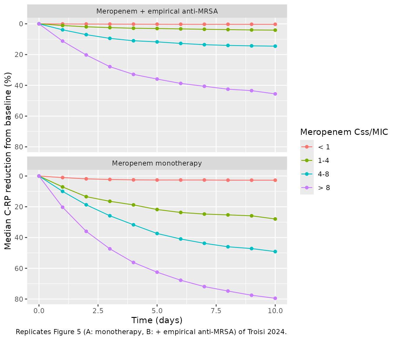
Comparison with the reported medians
paper_red <- tribble(
  ~group,                             ~target, ~day, ~paper,
  "Meropenem monotherapy",            "4-8",   2,    40,
  "Meropenem monotherapy",            "4-8",   4,    55,
  "Meropenem monotherapy",            "4-8",   10,   75,
  "Meropenem monotherapy",            "> 8",   10,   80,
  "Meropenem monotherapy",            "1-4",   2,    25,
  "Meropenem monotherapy",            "1-4",   4,    35,
  "Meropenem monotherapy",            "1-4",   10,   50,
  "Meropenem monotherapy",            "< 1",   4,    5,
  "Meropenem + empirical anti-MRSA",  "> 8",   10,   40,
  "Meropenem + empirical anti-MRSA",  "4-8",   10,   35,
  "Meropenem + empirical anti-MRSA",  "1-4",   10,   17,
  "Meropenem + empirical anti-MRSA",  "< 1",   10,   2
)
cmp_red <- paper_red |>
  left_join(mutate(crp_med, target = as.character(target)), by = c("group", "target", "day")) |>
  mutate(diff = median_red - paper)
cmp_red |>
  rename(Group = group, `Css/MIC` = target, Day = day,
         `Paper median reduction (%)` = paper,
         `Simulated median reduction (%)` = median_red,
         `Virtual patients` = n,
         `Difference (points)` = diff) |>
  knitr::kable(digits = 1,
caption = "Median C-RP reduction from baseline: Troisi 2024 Results text versus this simulation.")| Group | Css/MIC | Day | Paper median reduction (%) | Simulated median reduction (%) | Virtual patients | Difference (points) |
|---|---|---|---|---|---|---|
| Meropenem monotherapy | 4-8 | 2 | 40 | 18.7 | 96 | -21.3 |
| Meropenem monotherapy | 4-8 | 4 | 55 | 31.7 | 96 | -23.3 |
| Meropenem monotherapy | 4-8 | 10 | 75 | 49.1 | 96 | -25.9 |
| Meropenem monotherapy | > 8 | 10 | 80 | 79.5 | 661 | -0.5 |
| Meropenem monotherapy | 1-4 | 2 | 25 | 13.4 | 138 | -11.6 |
| Meropenem monotherapy | 1-4 | 4 | 35 | 18.8 | 138 | -16.2 |
| Meropenem monotherapy | 1-4 | 10 | 50 | 27.9 | 138 | -22.1 |
| Meropenem monotherapy | < 1 | 4 | 5 | 2.5 | 105 | -2.5 |
| Meropenem + empirical anti-MRSA | > 8 | 10 | 40 | 45.6 | 672 | 5.6 |
| Meropenem + empirical anti-MRSA | 4-8 | 10 | 35 | 14.5 | 93 | -20.5 |
| Meropenem + empirical anti-MRSA | 1-4 | 10 | 17 | 4.1 | 137 | -12.9 |
| Meropenem + empirical anti-MRSA | < 1 | 10 | 2 | 0.3 | 98 | -1.7 |
# The MIC and eGFR distributions behind the paper's 100,000 profiles are not
# reported, so the class medians can only be compared, not reproduced; the
# gate asserts the qualitative result instead. Each comparison below is between
# class medians that the paper separates by >= 25 points, and the per-class
# cohorts hold well over 100 patients. A mis-transcribed IC50, MIC or
# co-therapy coefficient would collapse or invert these gaps.
m <- function(g, t, d) crp_med$median_red[crp_med$group == g & crp_med$target == t & crp_med$day == d]
mono <- "Meropenem monotherapy"
mrsa <- "Meropenem + empirical anti-MRSA"
stopifnot(
  m(mono, "4-8", 10) - m(mono, "< 1", 10) > 25,
  m(mono, "4-8", 10) - m(mrsa, "4-8", 10) > 10,
  m(mono, "< 1", 4) < 25
)
The simulation reproduces the ordering the paper reports: C-RP falls
with rising Css/MIC, a sub-optimal ratio (< 1) leaves C-RP almost
unchanged, and empirical anti-MRSA co-therapy (which multiplies the IC50
by exp(2.46) = 11.7) flattens every class. The
supra-optimal (> 8) and sub-optimal (< 1) medians agree with the
paper within about 6 points. The quasi-optimal (1-4) and optimal (4-8)
medians come out 12-26 points lower than the paper’s.
Those two classes are sensitive to the cohort design, because the MIC
enters the model twice: through the Css/MIC ratio that defines the
class, and directly in the IC50 (exp(0.44 x MIC)). At a low
MIC a ratio of 4-8 means a Css of only 0.5-2 mg/L, close to the typical
IC50 of 0.79 mg/L, so inhibition is partial; at a high MIC the IC50
itself rises (34-fold at 8 mg/L). The median of a class therefore
depends on which MICs fill it, and the paper does not report how MIC was
assigned in its simulations. The breakdown below shows the spread within
the monotherapy 4-8 class.
crp_red |>
  filter(group == mono, target == "4-8", day == 10) |>
  group_by(MIC) |>
  summarise(`Virtual patients` = n(), `Median C-RP reduction at day 10 (%)` = median(pct_red),
            .groups = "drop") |>
  mutate(MIC = format(MIC, drop0trailing = TRUE)) |>
  rename(`MIC (mg/L)` = MIC) |>
  knitr::kable(digits = 1,
caption = "Monotherapy, Css/MIC 4-8: day-10 median C-RP reduction by isolate MIC.")| MIC (mg/L) | Virtual patients | Median C-RP reduction at day 10 (%) |
|---|---|---|
| 0.125 | 14 | 26.1 |
| 0.25 | 6 | 36.6 |
| 0.5 | 3 | 78.4 |
| 1 | 10 | 59.8 |
| 2 | 13 | 63.4 |
| 4 | 27 | 57.7 |
| 8 | 17 | 47.0 |
| 16 | 6 | 9.4 |
PKNCA validation
Meropenem is given by continuous infusion, so the useful NCA quantity
is the average steady-state concentration over the last simulated day
(216-240 h), which must equal rate / CL. The NCA is run on
the monotherapy arms (the PK is identical in both groups), grouped by
dosage.
conc_nca <- sim |>
  filter(CONMED_ANTIMRSA == 0, time >= 216, !is.na(Cc)) |>
  left_join(distinct(cohort, id, regimen), by = "id") |>
  mutate(treatment = regimen) |>
  select(id, time, Cc, treatment)
dose_nca <- cohort |>
  filter(CONMED_ANTIMRSA == 0) |>
  transmute(id, time = 216, amt = daily_mg, treatment = regimen)

conc_obj <- PKNCA::PKNCAconc(conc_nca, Cc ~ time | treatment + id)
dose_obj <- PKNCA::PKNCAdose(dose_nca, amt ~ time | treatment + id)
intervals <- data.frame(start = 216, end = 240, cav = TRUE, cmax = TRUE, cmin = TRUE)
# Linear trapezoid: at steady state of a constant-rate infusion the profile is
# flat, and the default lin-up/log-down rule evaluates (C1 - C2) / log(C1 / C2)
# on concentrations that differ only by floating-point rounding, which inflates
# the AUC by several percent for some subjects.
nca_res <- PKNCA::pk.nca(PKNCA::PKNCAdata(conc_obj, dose_obj, intervals = intervals,
                                          options = list(auc.method = "linear")))
nca_wide <- as.data.frame(nca_res) |>
  select(treatment, id, PPTESTCD, PPORRES) |>
  tidyr::pivot_wider(names_from = PPTESTCD, values_from = PPORRES) |>
  left_join(css_ind, by = "id")
summary(nca_res)
#>  start end   treatment   N        cmax        cmin         cav
#>    216 240 1000 mg q6h 200 26.3 [84.3] 26.3 [84.3] 26.3 [84.3]
#>    216 240  125 mg q8h 200 2.49 [97.7] 2.49 [97.7] 2.49 [97.7]
#>    216 240 1500 mg q6h 200 40.8 [82.8] 40.8 [82.8] 40.8 [82.8]
#>    216 240  500 mg q6h 200 12.8 [85.1] 12.8 [85.1] 12.8 [85.1]
#>    216 240  500 mg q8h 200 9.16 [86.1] 9.16 [86.1] 9.16 [86.1]
#>
#> Caption: cmax, cmin, cav: geometric mean and geometric coefficient of variation; N: number of subjects

# Closed-form identity: a constant-rate infusion started at time 0 gives
# C(t) = (rate / CL) * (1 - exp(-k t)), k = CL / V, so the exact average over
# 216-240 h is (rate / CL) * (1 - (exp(-216 k) - exp(-240 k)) / (24 k)).
# This keeps the check exact for the slowest clearers, which are not yet at
# steady state. Realised maximum deviation 7e-7 (solver tolerance).
cl_ind <- sim |> filter(time == 240) |> select(id, cl)
nca_wide <- nca_wide |>
  left_join(cl_ind, by = "id") |>
  left_join(distinct(cohort, id, daily_mg), by = "id") |>
  mutate(
    k = cl / exp(th[["lvc"]]),
    cav_closed = daily_mg / 24 / cl * (1 - (exp(-216 * k) - exp(-240 * k)) / (24 * k)),
    dev = cav / cav_closed - 1
  )
stopifnot(max(abs(nca_wide$dev)) < 1e-4)
The paper’s only observed exposure summary is the Table 1 median Css of 15.9 mg/L (IQR 9.8-27.6) at a median daily dose of 2 g. The table below sets the 2 g/day (500 mg q6h) arm against it; this arm’s eGFR spans 5-150 rather than the cohort’s IQR of 39-100, and the observed Css pools all doses, so it is a plausibility check rather than a reproduction.
published_nca <- tibble::tribble(
  ~treatment,     ~cav,
  "500 mg q6h",   15.9
)
cmp_nca <- nlmixr2lib::ncaComparisonTable(
  simulated = nca_res,
  reference = published_nca,
  by = "treatment",
  params = "cav",
  units = c(cav = "mg/L"),
  tolerance_pct = 20
)
knitr::kable(cmp_nca,
caption = "Simulated steady-state Cav versus Troisi 2024 Table 1 median Css. * differs from reference by >20%.")| NCA parameter | treatment | Reference | Simulated | % diff |
|---|---|---|---|---|
| Cavg (mg/L) | 500 mg q6h | 15.9 | 13 | -18.1% |
Assumptions and deviations
- Simulation MIC and eGFR distributions. The Monte Carlo methods list the dosages and renal classes but not how isolate MICs (or eGFR within a class) were assigned. This vignette draws MIC from the dilution series with weights matched to the Table 2 median and IQR, and eGFR uniformly within each class; the Css/MIC class medians therefore differ from Figure 5, and the comparison above is qualitative.
- Loading dose. The simulations start the maintenance infusion at time 0 without the clinical 2 g loading dose, following the dosage list in Methods. With V = 20 L and CL of 2.8-14 L/h, meropenem reaches steady state within hours, so the C-RP time course is barely affected.
- “Over 8 h” infusions given q6h. The Methods list 500 mg, 1000 mg and 1500 mg q6h “over 8 h”; these are encoded as continuous infusions delivering the stated daily dose at a constant rate.
- Sequential fit. The PK parameters were estimated first and then fixed while the PD parameters were fitted; the packaged model carries both sets at their reported final values, which is what the authors simulated from.
-
eGFR column. Table 3 labels the clearance covariate
‘CLCR’, but the Results equation, the ESM and the Methods all identify
it as CKD-EPI eGFR in mL/min/1.73 m^2, so it is stored as
CRCL. - Model scope. The PD model was fitted only to meropenem monotherapy and meropenem plus an empirical anti-MRSA agent. Patients receiving a second anti-Gram-negative agent or targeted anti-MRSA therapy contributed to the PK model only; the C-RP model is not defined for them.
- Uncentered exponential covariates. At high MIC the IC50 becomes very large (about 1100-fold at 16 mg/L), which is how the model represents an almost absent C-RP response to a resistant isolate. Results outside the published MIC range (0.12-64 mg/L) and eGFR range should not be extrapolated.
- Not retained covariates. Age, sex, weight, height and serum creatinine (on PK) and isolate type (P. aeruginosa versus other Gram-negative pathogens, on PD) were screened and not retained.