Rat neuro-PBPK for six drugs from three BBB cell lines (Sanchez-Dengra 2021)

library(nlmixr2lib)
library(rxode2)
library(PKNCA)
library(dplyr)
library(tidyr)
library(ggplot2)

The paper

Sanchez-Dengra and colleagues coupled a single in vitro blood-brain barrier (BBB) assay to a small semi-physiological PBPK model to predict drug concentrations in the rat brain. Three cell lines were used for the in vitro assay – MDCK, MDCK-MDR1 (MDCK transfected with human P-glycoprotein) and the human brain endothelial line hCMEC/D3 – and six model drugs were studied: amitriptyline, caffeine, carbamazepine, fleroxacin, pefloxacin and zolpidem.

Sanchez-Dengra B, Gonzalez-Alvarez I, Bermejo M, Gonzalez-Alvarez M. Physiologically Based Pharmacokinetic (PBPK) Modeling for Predicting Brain Levels of Drug in Rat. Pharmaceutics. 2021;13(9):1402. doi:10.3390/pharmaceutics13091402

• Article (open access): https://doi.org/10.3390/pharmaceutics13091402
• Supplement (Tables S1-S2): https://www.mdpi.com/article/10.3390/pharmaceutics13091402/s1

For every drug and every cell line the authors fitted the model to published mean plasma and brain profiles in Berkeley Madonna, estimating the plasma volume of distribution Vd, the elimination rate constant kel, the absorption rate constant ka (extravascular doses only) and three scaling factors that carry the in vitro inputs over to the rat (Table 3). The paper therefore reports 18 fitted parameterisations (six drugs times three cell lines) of one shared structure. Each is a separate model in this package:

drugs <- c("amitriptyline", "caffeine", "carbamazepine", "fleroxacin", "pefloxacin", "zolpidem")
cells <- c(mdck = "MDCK", mdckmdr1 = "MDCK-MDR1", hcmec = "hCMEC/D3")
grid <- expand.grid(cell = names(cells), drug = drugs, stringsAsFactors = FALSE)
grid$model <- sprintf("SanchezDengra_2021_%s_rat_pbpk_%s", grid$drug, grid$cell)
grid$cell_label <- factor(unname(cells[grid$cell]), levels = cells)
stopifnot(nrow(grid) == 18L, all(grid$model %in% modeldb$name))
mods <- lapply(setNames(grid$model, grid$model), function(m) rxode2::rxode(readModelDb(m)))
grid[, c("model", "drug", "cell_label")]
#>                                                 model          drug cell_label
#> 1      SanchezDengra_2021_amitriptyline_rat_pbpk_mdck amitriptyline       MDCK
#> 2  SanchezDengra_2021_amitriptyline_rat_pbpk_mdckmdr1 amitriptyline  MDCK-MDR1
#> 3     SanchezDengra_2021_amitriptyline_rat_pbpk_hcmec amitriptyline   hCMEC/D3
#> 4           SanchezDengra_2021_caffeine_rat_pbpk_mdck      caffeine       MDCK
#> 5       SanchezDengra_2021_caffeine_rat_pbpk_mdckmdr1      caffeine  MDCK-MDR1
#> 6          SanchezDengra_2021_caffeine_rat_pbpk_hcmec      caffeine   hCMEC/D3
#> 7      SanchezDengra_2021_carbamazepine_rat_pbpk_mdck carbamazepine       MDCK
#> 8  SanchezDengra_2021_carbamazepine_rat_pbpk_mdckmdr1 carbamazepine  MDCK-MDR1
#> 9     SanchezDengra_2021_carbamazepine_rat_pbpk_hcmec carbamazepine   hCMEC/D3
#> 10        SanchezDengra_2021_fleroxacin_rat_pbpk_mdck    fleroxacin       MDCK
#> 11    SanchezDengra_2021_fleroxacin_rat_pbpk_mdckmdr1    fleroxacin  MDCK-MDR1
#> 12       SanchezDengra_2021_fleroxacin_rat_pbpk_hcmec    fleroxacin   hCMEC/D3
#> 13        SanchezDengra_2021_pefloxacin_rat_pbpk_mdck    pefloxacin       MDCK
#> 14    SanchezDengra_2021_pefloxacin_rat_pbpk_mdckmdr1    pefloxacin  MDCK-MDR1
#> 15       SanchezDengra_2021_pefloxacin_rat_pbpk_hcmec    pefloxacin   hCMEC/D3
#> 16          SanchezDengra_2021_zolpidem_rat_pbpk_mdck      zolpidem       MDCK
#> 17      SanchezDengra_2021_zolpidem_rat_pbpk_mdckmdr1      zolpidem  MDCK-MDR1
#> 18         SanchezDengra_2021_zolpidem_rat_pbpk_hcmec      zolpidem   hCMEC/D3

The models are deterministic: the paper fitted mean profiles and estimated no between-animal variability and no residual error, so there are no eta or residual-error terms, and every simulation below is a single typical-value solve.

Model structure

Figure 1 of the paper has one plasma compartment (central, volume Vd) and two CNS compartments: brain tissue (brain, volume Vb) and cerebrospinal fluid (csf, volume VCSF). Only unbound drug crosses a barrier. For total concentrations Cp (plasma) and Cb (brain) and the CSF concentration CCSF, Equations 4-6 are

Vd   dCp/dt   = - PS_BBB,in Cu,p + PS_BBB,out Cu,b - PS_BCSFB,in Cu,p
                + PS_BCSFB,out CCSF + Qsink CCSF - kel Cp Vd
Vb   dCb/dt   =   PS_BBB,in Cu,p - PS_BBB,out Cu,b - Qbulk Cu,b
VCSF dCCSF/dt =   PS_BCSFB,in Cu,p - PS_BCSFB,out CCSF - Qsink CCSF + Qbulk Cu,b

with the unbound concentrations Cu,p = fu,plasma Cp (Figure 1) and Cu,b = SC3 fu,brain Cb (Equation 14), all CSF drug unbound, and the barrier permeability-surface-area products built from the in vitro apparent permeabilities (Equations 10-13):

PS_BBB,in    = SC1 Papp,A-B S_BBB      PS_BCSFB,in  = SC1 Papp,A-B S_BCSFB
PS_BBB,out   = SC2 Papp,B-A S_BBB      PS_BCSFB,out = SC2 Papp,B-A S_BCSFB

An extravascular dose adds a depot dA/dt = -ka A feeding plasma at ka A (Equations 7-8); an intravenous infusion adds the zero-order input k0 (Equation 9), which the package models supply as an infusion event rather than as a term in the ODE. Nothing is eliminated from the brain or the CSF: every molecule that enters the CNS returns to plasma, and kel is the only exit from the system.

Population

The in vivo data are literature mean profiles (Methods 2.4, references 16-20), one rat study per drug, so the paper reports no number of animals. The rat weights of the source studies were 190-300 g (Table 1). The brain data are total brain concentrations for amitriptyline and zolpidem and unbound brain (or brain extracellular fluid) concentrations for the other four drugs; the plasma data are total plasma concentrations except for carbamazepine, whose plasma profile is unbound (Figure 2 legends). The same information is in each model’s population metadata:

str(readModelDb("SanchezDengra_2021_caffeine_rat_pbpk_mdck")()$population)
#> List of 8
#>  $ species        : chr "rat"
#>  $ n_subjects     : int NA
#>  $ n_studies      : int 1
#>  $ weight_range   : chr "300 g (Table 1)"
#>  $ disease_state  : chr "healthy"
#>  $ dose_range     : chr "constant-rate intravenous infusion at k0 = 833.333 ng/s (Table 1 k0; Equation 9)"
#>  $ in_vitro_system: chr "MDCK (Madin-Darby canine kidney) transwell monolayers; fu,brain from pig brain homogenate"
#>  $ notes          : chr "The caffeine plasma and brain concentration-time profiles were taken from the published literature (Methods 2.4"| __truncated__

Source trace

Every ini() value carries an in-file comment naming its source. They are collected here.

Quantity	Symbol in model	Source
Model structure	d/dt(central), d/dt(brain), d/dt(csf)	Figure 1; Equations 4-6
Extravascular input	d/dt(depot), ka	Equations 7-8
Infusion input	infusion event into central	Equation 9
Barrier PS products	ps_bbb_in, ps_bbb_out, ps_bcsfb_in, ps_bcsfb_out	Equations 10-13
Unbound brain concentration	Cu_brain <- sc3 * fu_brain * Cbrain	Equation 14
Unbound plasma concentration	Cu <- fu * Cc	Figure 1
Vd, kel, ka (fitted)	lvc, lkel, lka	Table 3 (Table 1 holds the initial estimates)
SC1, SC2, SC3 per cell line (fitted)	sc1, sc2, sc3	Table 3
Papp,A-B, Papp,B-A, fu,brain per cell line (fixed)	papp_ab, papp_ba, fu_brain	Table 2
fu,plasma (fixed)	fu	Table 1
Vb = 1.28 cm^3, VCSF = 0.25 cm^3	lvbrain, lvcsf	Methods 2.4 (Ball et al., ref 14)
Qbulk = 0.012 cm^3/s, Qsink = 0.132 cm^3/s	qbulk, qsink	Methods 2.4 (Ball et al., ref 14)
S_BBB = 187.5 cm^2, S_BCSFB = 0.0375 cm^2	s_bbb, s_bcsfb	Methods 2.4 (ref 14; Engelhard et al., ref 15)
Doses D, infusion rates k0, rat weights	event tables below	Table 1
QSPR polynomials lnSC = f(logP)	vignette only	Figure 3 (printed equations)
logP of each drug	vignette only	Supplementary Table S2

The eighteen files differ only in the Table 1-3 values. The parameter values of all eighteen, read back out of the packaged models:

param_row <- function(m) {
  ini <- mods[[m]]$iniDf
  v <- setNames(ini$est, ini$name)
  data.frame(
    model = m,
    Vd_mL = exp(v[["lvc"]]),
    kel_per_s = signif(exp(v[["lkel"]]), 3),
    ka_per_s = if ("lka" %in% names(v)) signif(exp(v[["lka"]]), 3) else NA_real_,
    fu_plasma = v[["fu"]],
    Papp_AB = v[["papp_ab"]],
    Papp_BA = v[["papp_ba"]],
    fu_brain = v[["fu_brain"]],
    SC1 = v[["sc1"]],
    SC2 = v[["sc2"]],
    SC3 = v[["sc3"]]
  )
}
params <- do.call(rbind, lapply(grid$model, param_row))
knitr::kable(params, row.names = FALSE)

model	Vd_mL	kel_per_s	ka_per_s	fu_plasma	Papp_AB	Papp_BA	fu_brain	SC1	SC2	SC3
SanchezDengra_2021_amitriptyline_rat_pbpk_mdck	14632.6	1.17e-04	0.005860	0.090	74.77	178.48	0.037	220.59	224.82	0.05
SanchezDengra_2021_amitriptyline_rat_pbpk_mdckmdr1	14632.6	1.17e-04	0.005860	0.090	17.95	16.91	0.104	920.39	2377.06	0.02
SanchezDengra_2021_amitriptyline_rat_pbpk_hcmec	14632.6	1.17e-04	0.005860	0.090	124.24	66.21	0.252	132.89	606.69	0.01
SanchezDengra_2021_caffeine_rat_pbpk_mdck	273.6	3.55e-05	NA	0.917	26.10	35.31	0.857	3.85	1.00	0.22
SanchezDengra_2021_caffeine_rat_pbpk_mdckmdr1	273.6	3.55e-05	NA	0.917	33.57	30.59	0.613	2.85	1.00	0.31
SanchezDengra_2021_caffeine_rat_pbpk_hcmec	273.6	3.55e-05	NA	0.917	63.93	194.70	0.095	4.09	1.00	2.15
SanchezDengra_2021_carbamazepine_rat_pbpk_mdck	827.0	5.39e-05	0.000215	0.385	114.64	78.66	0.673	25.71	81.01	1.16
SanchezDengra_2021_carbamazepine_rat_pbpk_mdckmdr1	827.0	5.39e-05	0.000215	0.385	142.96	75.64	0.238	95.00	391.22	0.71
SanchezDengra_2021_carbamazepine_rat_pbpk_hcmec	827.0	5.39e-05	0.000215	0.385	70.14	51.93	0.386	193.66	569.98	0.44
SanchezDengra_2021_fleroxacin_rat_pbpk_mdck	327.3	2.69e-05	NA	0.793	88.48	63.44	0.471	3.18	12.96	1.07
SanchezDengra_2021_fleroxacin_rat_pbpk_mdckmdr1	327.3	2.69e-05	NA	0.793	67.40	42.57	0.813	1.59	6.43	0.68
SanchezDengra_2021_fleroxacin_rat_pbpk_hcmec	327.3	2.69e-05	NA	0.793	29.96	25.73	0.743	3.58	10.65	0.74
SanchezDengra_2021_pefloxacin_rat_pbpk_mdck	524.3	6.75e-05	NA	0.860	41.21	37.49	0.910	4.88	13.32	0.55
SanchezDengra_2021_pefloxacin_rat_pbpk_mdckmdr1	524.3	6.75e-05	NA	0.860	30.82	35.39	0.931	6.15	13.19	0.56
SanchezDengra_2021_pefloxacin_rat_pbpk_hcmec	524.3	6.75e-05	NA	0.860	24.95	33.14	0.642	7.59	14.09	0.81
SanchezDengra_2021_zolpidem_rat_pbpk_mdck	185.9	5.12e-04	NA	0.267	21.32	36.48	0.971	16.53	26.79	0.27
SanchezDengra_2021_zolpidem_rat_pbpk_mdckmdr1	185.9	5.12e-04	NA	0.267	8.92	33.43	0.881	20.59	14.51	0.30
SanchezDengra_2021_zolpidem_rat_pbpk_hcmec	185.9	5.12e-04	NA	0.267	106.16	80.76	0.408	10.26	38.70	0.65

Dosing designs (Table 1)

Table 1 gives, per drug, a dose D and/or an infusion rate k0. Read together with Figure 2 the designs are:

• Amitriptyline and carbamazepine – a single extravascular dose D (5,000,000 ng and 3,600,000 ng) with first-order absorption ka.
• Zolpidem – a single intravenous bolus D = 499,700 ng; D / Vd = 2688 ng/mL is the fitted plasma line’s value at time zero in Figure 2F.
• Fleroxacin and pefloxacin – an intravenous loading bolus D followed by a constant infusion k0 for the whole 14,400 s record. Both D and k0 are printed; that D is a bolus at time zero is confirmed by D / Vd = 3405 and 7012 ng/mL, the fitted plasma lines’ starting values in Figure 2D and 2E.
• Caffeine – a constant infusion k0 = 833.333 ng/s with no bolus. The paper does not print the infusion duration; it is taken as 14,400 s (4 h), where the fitted plasma and brain lines of Figure 2B peak.

design <- data.frame(
  drug = drugs,
  bolus_amt = c(5e6, 0, 3.6e6, 1114350, 3676500, 499700),
  bolus_cmt = c("depot", "central", "depot", "central", "central", "central"),
  inf_rate = c(0, 833.333, 0, 83.125, 214.542, 0),
  inf_dur = c(0, 14400, 0, 14400, 14400, 0),
  t_end = c(86400, 28800, 50400, 14400, 14400, 21600),
  stringsAsFactors = FALSE
)
# Which concentrations Figure 2 plots for each drug (legends of Figure 2)
design$plasma_var <- c("Cc", "Cc", "Cu", "Cc", "Cc", "Cc")
design$brain_var <- c("Cbrain", "Cu_brain", "Cu_brain", "Cu_brain", "Cu_brain", "Cbrain")
knitr::kable(design)

drug	bolus_amt	bolus_cmt	inf_rate	inf_dur	t_end	plasma_var	brain_var
amitriptyline	5000000	depot	0.000	0	86400	Cc	Cbrain
caffeine	0	central	833.333	14400	28800	Cc	Cu_brain
carbamazepine	3600000	depot	0.000	0	50400	Cu	Cu_brain
fleroxacin	1114350	central	83.125	14400	14400	Cc	Cu_brain
pefloxacin	3676500	central	214.542	14400	14400	Cc	Cu_brain
zolpidem	499700	central	0.000	0	21600	Cc	Cbrain

make_events <- function(drug, obs_times) {
  d <- design[design$drug == drug, ]
  ev <- rxode2::et(obs_times, cmt = "central")
  if (d$bolus_amt > 0) {
    ev <- rxode2::et(ev, amt = d$bolus_amt, cmt = d$bolus_cmt, time = 0)
  }
  if (d$inf_rate > 0) {
    ev <- rxode2::et(ev, amt = d$inf_rate * d$inf_dur, rate = d$inf_rate, cmt = "central", time = 0)
  }
  ev
}

solve_one <- function(m, drug, obs_times, ...) {
  s <- as.data.frame(rxode2::rxSolve(mods[[m]], make_events(drug, obs_times), ...))
  s$model <- m
  s
}

Replicating Figure 2: the fitted profiles

Each fitted parameterisation is solved on the design of its source study. The panels plot the same quantities as Figure 2 of the paper (total or unbound, as in its legends).

fig2 <- lapply(seq_len(nrow(grid)), function(i) {
  d <- design[design$drug == grid$drug[i], ]
  obs <- sort(unique(c(seq(0, d$t_end, length.out = 401), 1:120)))
  obs <- obs[obs <= d$t_end]
  s <- solve_one(grid$model[i], grid$drug[i], obs)
  data.frame(
    drug = grid$drug[i], cell = grid$cell_label[i], time = s$time,
    plasma = s[[d$plasma_var]], brain = s[[d$brain_var]]
  )
})
fig2 <- do.call(rbind, fig2)
fig2_long <- fig2 |>
  pivot_longer(c(plasma, brain), names_to = "matrix", values_to = "conc") |>
  mutate(matrix = factor(matrix, levels = c("plasma", "brain")))

ggplot(fig2_long, aes(time, conc, colour = cell)) +
  geom_line() +
  facet_wrap(drug ~ matrix, scales = "free", ncol = 4) +
  labs(x = "t (s)", y = "C (ng/mL)", colour = "Cell line") +
  theme_bw() +
  theme(legend.position = "bottom")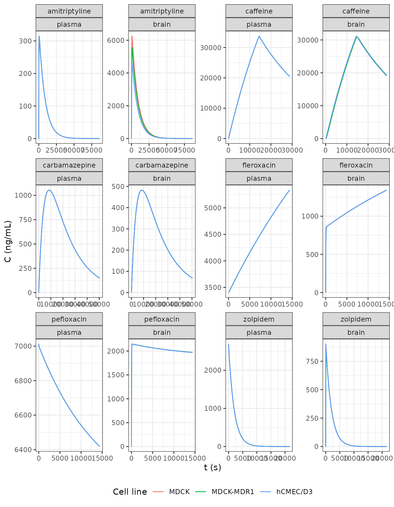

Replicates Figure 2 of Sanchez-Dengra 2021: fitted plasma and brain profiles for each drug and cell line (the three cell-line fits overlap, as in the paper).

The fitted lines of Figure 2 were read by eye at the points below (fitted-line peaks, or the start and end of the constant-infusion records). They are visual reads of a printed figure, so the check allows 15 percent – enough for the reading error, and far too little for a wrong dose, volume or unit, which move these values several-fold. The check uses the MDCK fit, the cell line the paper recommends; the next check covers the other two.

anchor <- data.frame(
  drug = c(
    "amitriptyline", "amitriptyline", "caffeine", "caffeine", "carbamazepine",
    "carbamazepine", "fleroxacin", "fleroxacin", "pefloxacin", "pefloxacin",
    "zolpidem", "zolpidem"
  ),
  matrix = c(
    "plasma", "brain", "plasma", "brain", "plasma", "brain",
    "plasma", "brain", "plasma", "brain", "plasma", "brain"
  ),
  what = c(
    "peak", "peak", "peak", "peak", "peak", "peak",
    "end", "end", "end", "end", "start", "peak"
  ),
  figure2 = c(310, 6000, 34000, 30500, 1050, 490, 5400, 1380, 6400, 2000, 2700, 880)
)
sim_at <- function(drug, matrix, what) {
  x <- fig2_long[fig2_long$drug == drug & fig2_long$matrix == matrix & fig2_long$cell == "MDCK", ]
  if (nrow(x) == 0L) stop("no simulated rows for ", drug, " ", matrix)
  switch(what,
    peak = max(x$conc),
    start = x$conc[which.min(x$time)],
    end = x$conc[which.max(x$time)]
  )
}
anchor$simulated <- mapply(sim_at, anchor$drug, anchor$matrix, anchor$what)
anchor$pct_diff <- round(100 * (anchor$simulated / anchor$figure2 - 1), 1)
anchor$simulated <- signif(anchor$simulated, 4)
knitr::kable(anchor)

drug	matrix	what	figure2	simulated	pct_diff
amitriptyline	plasma	peak	310	314.9	1.6
amitriptyline	brain	peak	6000	6255.0	4.3
caffeine	plasma	peak	34000	33750.0	-0.7
caffeine	brain	peak	30500	30940.0	1.4
carbamazepine	plasma	peak	1050	1055.0	0.4
carbamazepine	brain	peak	490	483.0	-1.4
fleroxacin	plasma	end	5400	5336.0	-1.2
fleroxacin	brain	end	1380	1343.0	-2.7
pefloxacin	plasma	end	6400	6418.0	0.3
pefloxacin	brain	end	2000	1970.0	-1.5
zolpidem	plasma	start	2700	2688.0	-0.4
zolpidem	brain	peak	880	873.7	-0.7

stopifnot(nrow(anchor) == 12L, all(abs(anchor$pct_diff) < 15))

The paper states that the three cell-line fits overlap in both plasma and brain (Figure 2 and Discussion). Brain exposure of the MDCK-MDR1 and hCMEC/D3 fits, relative to the MDCK fit of the same drug:

overlap <- fig2 |>
  group_by(drug, cell) |>
  summarise(
    brain_auc = sum(diff(time) * (head(brain, -1) + tail(brain, -1)) / 2),
    brain_cmax = max(brain),
    .groups = "drop"
  ) |>
  group_by(drug) |>
  mutate(
    auc_vs_mdck_pct = round(100 * (brain_auc / brain_auc[cell == "MDCK"] - 1), 1),
    cmax_vs_mdck_pct = round(100 * (brain_cmax / brain_cmax[cell == "MDCK"] - 1), 1)
  ) |>
  ungroup()
overlap$deviation <- overlap$drug == "amitriptyline" & overlap$cell != "MDCK"
knitr::kable(overlap |> select(drug, cell, auc_vs_mdck_pct, cmax_vs_mdck_pct, deviation))

drug	cell	auc_vs_mdck_pct	cmax_vs_mdck_pct	deviation
amitriptyline	MDCK	0.0	0.0	FALSE
amitriptyline	MDCK-MDR1	-11.1	-11.0	TRUE
amitriptyline	hCMEC/D3	-26.6	-26.5	TRUE
caffeine	MDCK	0.0	0.0	FALSE
caffeine	MDCK-MDR1	-0.1	-0.1	FALSE
caffeine	hCMEC/D3	0.8	0.8	FALSE
carbamazepine	MDCK	0.0	0.0	FALSE
carbamazepine	MDCK-MDR1	0.0	-0.1	FALSE
carbamazepine	hCMEC/D3	0.0	-0.1	FALSE
fleroxacin	MDCK	0.0	0.0	FALSE
fleroxacin	MDCK-MDR1	-0.2	-0.1	FALSE
fleroxacin	hCMEC/D3	-0.2	-0.1	FALSE
pefloxacin	MDCK	0.0	0.0	FALSE
pefloxacin	MDCK-MDR1	0.0	0.0	FALSE
pefloxacin	hCMEC/D3	-0.1	-0.1	FALSE
zolpidem	MDCK	0.0	0.0	FALSE
zolpidem	MDCK-MDR1	-2.0	-5.5	FALSE
zolpidem	hCMEC/D3	-0.2	3.2	FALSE

# Measured within 2.0 percent for every row not flagged as a deviation.
stopifnot(nrow(overlap) == 18L, sum(overlap$deviation) == 2L, all(abs(overlap$auc_vs_mdck_pct[!overlap$deviation]) < 5))

The fits overlap for five of the six drugs. For amitriptyline the MDCK-MDR1 and hCMEC/D3 total brain profiles lie 11 and 27 percent below the MDCK one, whereas all three overlap in Figure 2A. This is a known deviation, and it comes from rounding in Table 3. Amitriptyline is extensively bound in brain, and the fitted SC3 values are printed to two decimals as 0.05, 0.02 and 0.01. The unbound brain concentration is fixed by the barrier permeabilities, so the three fits agree on it (checked below). The total concentration is the unbound one divided by SC3 * fu,brain, which as printed is 0.00185, 0.00208 and 0.00252 for the three cell lines. For the total profiles to overlap as they do in the paper, the unrounded hCMEC/D3 SC3 must be about 0.0073, not 0.01. The Figure 3C point for amitriptyline sits at ln SC3 of about -4.9 (SC3 of about 0.0075), which agrees. The packaged models keep the printed 0.02 and 0.01. The check below confirms that this is the whole explanation: the unbound profiles overlap, and the ratio of the total-brain AUCs equals the ratio of the printed SC3 * fu,brain products.

ami <- lapply(grid$model[grid$drug == "amitriptyline"], function(m) {
  s <- solve_one(m, "amitriptyline", seq(0, 86400, by = 60))
  v <- params[params$model == m, ]
  data.frame(
    model = m,
    auc_unbound = sum(diff(s$time) * (head(s$Cu_brain, -1) + tail(s$Cu_brain, -1)) / 2),
    auc_total = sum(diff(s$time) * (head(s$Cbrain, -1) + tail(s$Cbrain, -1)) / 2),
    binding = v$SC3 * v$fu_brain
  )
})
ami <- do.call(rbind, ami)
ami$unbound_vs_mdck <- ami$auc_unbound / ami$auc_unbound[1]
ami$total_vs_mdck <- ami$auc_total / ami$auc_total[1]
ami$binding_ratio <- ami$binding[1] / ami$binding
knitr::kable(ami, digits = 4)

model	auc_unbound	auc_total	binding	unbound_vs_mdck	total_vs_mdck	binding_ratio
SanchezDengra_2021_amitriptyline_rat_pbpk_mdck	107865.4	58305618	0.0019	1.0000	1.0000	1.0000
SanchezDengra_2021_amitriptyline_rat_pbpk_mdckmdr1	107856.7	51854182	0.0021	0.9999	0.8894	0.8894
SanchezDengra_2021_amitriptyline_rat_pbpk_hcmec	107859.2	42801253	0.0025	0.9999	0.7341	0.7341

stopifnot(
  nrow(ami) == 3L, grepl("_mdck$", ami$model[1]),
  all(abs(ami$unbound_vs_mdck - 1) < 0.02),
  all(abs(ami$total_vs_mdck / ami$binding_ratio - 1) < 0.02)
)

Structural identities

Two properties of the structure hold exactly for every parameterisation, and test the ODEs and the unit handling independently of any figure.

Plasma AUC and the dose

Because the CNS returns everything to plasma, the total dose leaves the system only through kel, so kel * Vd * AUC(0-inf, total plasma) = total dose whatever the CNS parameters are. A mis-signed exchange term or a mis-scaled permeability would break it. The AUC is computed with PKNCA on a long, dense grid of each drug’s Table 1 design, grouped by drug and cell line.

ident <- lapply(seq_len(nrow(grid)), function(i) {
  ini <- mods[[grid$model[i]]]$iniDf
  kel <- exp(ini$est[ini$name == "lkel"])
  obs <- sort(unique(c(0, 10^seq(0, log10(40 * log(2) / kel), length.out = 800))))
  s <- solve_one(grid$model[i], grid$drug[i], obs, rtol = 1e-10, atol = 1e-10, maxsteps = 1e6)
  data.frame(treatment = paste(grid$drug[i], grid$cell[i], sep = "_"), id = 1L, time = s$time, Cc = s$Cc)
})
ident <- do.call(rbind, ident)
stopifnot(all(ident$Cc >= -1e-6 * max(ident$Cc)))
conc_ident <- ident |>
  filter(!is.na(Cc)) |>
  mutate(Cc = pmax(Cc, 0)) |>
  select(treatment, id, time, Cc)
dose_ident <- design |>
  mutate(total_dose = bolus_amt + inf_rate * inf_dur) |>
  select(drug, total_dose) |>
  right_join(grid |> select(drug, cell), by = "drug") |>
  mutate(treatment = paste(drug, cell, sep = "_"), id = 1L, time = 0)
o_conc <- PKNCAconc(conc_ident, Cc ~ time | treatment + id)
o_dose <- PKNCAdose(dose_ident, total_dose ~ time | treatment + id)
o_data <- PKNCAdata(o_conc, o_dose,
  intervals = data.frame(start = 0, end = Inf, aucinf.obs = TRUE),
  options = list(auc.method = "lin up/log down")
)
nca_ident <- as.data.frame(pk.nca(o_data))
auc_check <- nca_ident |>
  filter(PPTESTCD == "aucinf.obs") |>
  left_join(dose_ident |> select(treatment, total_dose, drug, cell), by = "treatment") |>
  left_join(params |> mutate(treatment = sub("^SanchezDengra_2021_(.*)_rat_pbpk_(.*)$", "\\1_\\2", model)),
    by = "treatment"
  ) |>
  mutate(ratio = kel_per_s * Vd_mL * PPORRES / total_dose)
knitr::kable(auc_check |> select(treatment, total_dose, aucinf = PPORRES, ratio), digits = 4)

treatment	total_dose	aucinf	ratio
amitriptyline_hcmec	5000000	2920534	1
amitriptyline_mdck	5000000	2920534	1
amitriptyline_mdckmdr1	5000000	2920534	1
caffeine_hcmec	11999995	1235469127	1
caffeine_mdck	11999995	1235469206	1
caffeine_mdckmdr1	11999995	1235469205	1
carbamazepine_hcmec	3600000	80761382	1
carbamazepine_mdck	3600000	80761381	1
carbamazepine_mdckmdr1	3600000	80761382	1
fleroxacin_hcmec	2311350	262521008	1
fleroxacin_mdck	2311350	262521008	1
fleroxacin_mdckmdr1	2311350	262521008	1
pefloxacin_hcmec	6765905	191178737	1
pefloxacin_mdck	6765905	191178737	1
pefloxacin_mdckmdr1	6765905	191178737	1
zolpidem_hcmec	499700	5250008	1
zolpidem_mdck	499700	5250008	1
zolpidem_mdckmdr1	499700	5250008	1

# The ratio is 1 up to the trapezoid and extrapolation error of the NCA
# (measured at most 1.1e-5 on this grid); a sign error in any exchange term
# or a 1e-6 unit slip moves it by far more than 0.5 percent.
stopifnot(nrow(auc_check) == 18L, all(abs(auc_check$ratio - 1) < 0.005))

kel_per_s above comes from signif(..., 3), which equals the printed Table 3 value exactly.

Steady-state brain partitioning

At steady state Equation 5 gives the unbound brain-to-plasma ratio directly: Kp,uu,brain = Cu,b / Cu,p = PS_BBB,in / (PS_BBB,out + Qbulk), and Equation 6 then gives CCSF / Cu,p = (PS_BCSFB,in + Qbulk Kp,uu) / (PS_BCSFB,out + Qsink). A long constant infusion drives each parameterisation to steady state, and the simulated ratios are compared with the closed forms.

kp <- lapply(seq_len(nrow(grid)), function(i) {
  v <- params[params$model == grid$model[i], ]
  kel <- v$kel_per_s
  t_ss <- 60 * log(2) / kel
  ev <- rxode2::et(amt = t_ss, rate = 1, cmt = "central", time = 0)
  ev <- rxode2::et(ev, t_ss * (1 - 1e-6), cmt = "central")
  s <- as.data.frame(rxode2::rxSolve(mods[[grid$model[i]]], ev, rtol = 1e-10, atol = 1e-12, maxsteps = 1e6))
  s <- s[nrow(s), ]
  ps_in <- v$SC1 * v$Papp_AB * 1e-6 * 187.5
  ps_out <- v$SC2 * v$Papp_BA * 1e-6 * 187.5
  kpuu <- ps_in / (ps_out + 0.012)
  csf_ratio <- (v$SC1 * v$Papp_AB * 1e-6 * 0.0375 + 0.012 * kpuu) /
    (v$SC2 * v$Papp_BA * 1e-6 * 0.0375 + 0.132)
  data.frame(
    model = grid$model[i],
    kpuu_closed = kpuu, kpuu_sim = s$Cu_brain / s$Cu,
    csf_closed = csf_ratio, csf_sim = s$Ccsf / s$Cu
  )
})
kp <- do.call(rbind, kp)
kp$kpuu_relerr <- kp$kpuu_sim / kp$kpuu_closed - 1
kp$csf_relerr <- kp$csf_sim / kp$csf_closed - 1
knitr::kable(kp, digits = 5)

model	kpuu_closed	kpuu_sim	csf_closed	csf_sim	kpuu_relerr	csf_relerr
SanchezDengra_2021_amitriptyline_rat_pbpk_mdck	0.41039	0.41039	0.04152	0.04152	0	0
SanchezDengra_2021_amitriptyline_rat_pbpk_mdckmdr1	0.41036	0.41036	0.04152	0.04152	0	0
SanchezDengra_2021_amitriptyline_rat_pbpk_hcmec	0.41037	0.41037	0.04152	0.04152	0	0
SanchezDengra_2021_caffeine_rat_pbpk_mdck	1.01183	1.01183	0.09201	0.09201	0	0
SanchezDengra_2021_caffeine_rat_pbpk_mdckmdr1	1.01147	1.01147	0.09198	0.09198	0	0
SanchezDengra_2021_caffeine_rat_pbpk_hcmec	1.01072	1.01072	0.09195	0.09195	0	0
SanchezDengra_2021_carbamazepine_rat_pbpk_mdck	0.45794	0.45794	0.04239	0.04239	0	0
SanchezDengra_2021_carbamazepine_rat_pbpk_mdckmdr1	0.45796	0.45796	0.04511	0.04511	0	0
SanchezDengra_2021_carbamazepine_rat_pbpk_hcmec	0.45792	0.45792	0.04511	0.04511	0	0
SanchezDengra_2021_fleroxacin_rat_pbpk_mdck	0.31750	0.31750	0.02894	0.02894	0	0
SanchezDengra_2021_fleroxacin_rat_pbpk_mdckmdr1	0.31732	0.31732	0.02888	0.02888	0	0
SanchezDengra_2021_fleroxacin_rat_pbpk_hcmec	0.31730	0.31730	0.02887	0.02887	0	0
SanchezDengra_2021_pefloxacin_rat_pbpk_mdck	0.35697	0.35697	0.03250	0.03250	0	0
SanchezDengra_2021_pefloxacin_rat_pbpk_mdckmdr1	0.35709	0.35709	0.03251	0.03251	0	0
SanchezDengra_2021_pefloxacin_rat_pbpk_hcmec	0.35667	0.35667	0.03247	0.03247	0	0
SanchezDengra_2021_zolpidem_rat_pbpk_mdck	0.33844	0.33844	0.03086	0.03086	0	0
SanchezDengra_2021_zolpidem_rat_pbpk_mdckmdr1	0.33450	0.33450	0.03046	0.03046	0	0
SanchezDengra_2021_zolpidem_rat_pbpk_hcmec	0.34151	0.34151	0.03133	0.03133	0	0

# Measured at most 4e-13 with rtol = 1e-10; 1e-5 leaves headroom for the
# numeric integrator while still failing on any structural or unit error.
stopifnot(nrow(kp) == 18L, all(abs(kp$kpuu_relerr) < 1e-5), all(abs(kp$csf_relerr) < 1e-5))

The steady-state Kp,uu,brain values sit near or below 1 for every drug. This is a property of the fitted parameters, not a structural constraint; Qbulk enters the denominator, so the packaged structure can in principle produce Kp,uu above 1 when PS_BBB,in is large.

Replicating Figure 3: the QSPR sub-model

To predict brain levels for a new drug, the authors regressed the natural logarithm of each fitted scaling factor on the drug’s lipophilicity (logP): a cubic for SC1 and SC2 and a parabola for SC3, separately for each cell line (Figure 3). The polynomial coefficients are printed under each panel of Figure 3 and the logP values are in Supplementary Table S2.

logp <- c(
  amitriptyline = 4.81, caffeine = -0.55, carbamazepine = 2.77,
  fleroxacin = 0.98, pefloxacin = 0.75, zolpidem = 3.02
)
# Coefficients (x^3, x^2, x, intercept) of Figure 3, one row per cell line and
# scaling factor, with the printed R^2.
qspr <- data.frame(
  cell = rep(c("mdck", "mdckmdr1", "hcmec"), each = 3),
  sc = rep(c("sc1", "sc2", "sc3"), times = 3),
  a3 = c(-0.019, 0.080, 0, -0.044, 0.083, 0, -0.055, 0.020, 0),
  a2 = c(0.284, -0.63, -0.291, 0.470, -0.488, -0.308, 0.380, -0.275, -0.247),
  a1 = c(-0.048, 2.016, 0.967, -0.020, 1.794, 0.844, 0.184, 1.946, 0.180),
  a0 = c(1.237, 1.300, -0.888, 0.903, 1.116, -0.779, 1.358, 1.125, 0.394),
  r2_printed = c(0.969, 0.955, 0.854, 0.894, 0.831, 0.959, 0.643, 0.855, 0.895),
  stringsAsFactors = FALSE
)
qspr_predict <- function(row, x) exp(row$a3 * x^3 + row$a2 * x^2 + row$a1 * x + row$a0)

qspr_check <- lapply(seq_len(nrow(qspr)), function(k) {
  q <- qspr[k, ]
  fitted_sc <- vapply(drugs, function(dr) {
    params[[toupper(q$sc)]][params$model == sprintf("SanchezDengra_2021_%s_rat_pbpk_%s", dr, q$cell)]
  }, numeric(1))
  y <- log(fitted_sc)
  yhat <- log(qspr_predict(q, logp[drugs]))
  refit <- lm(y ~ poly(logp[drugs], if (q$sc == "sc3") 2 else 3, raw = TRUE))
  data.frame(
    cell = q$cell, sc = q$sc, r2_printed = q$r2_printed,
    r2_printed_coefs = 1 - sum((y - yhat)^2) / sum((y - mean(y))^2),
    r2_refit = summary(refit)$r.squared,
    max_coef_diff = max(abs(rev(coef(refit)) - c(q$a3, q$a2, q$a1, q$a0)[if (q$sc == "sc3") 2:4 else 1:4]))
  )
})
qspr_check <- do.call(rbind, qspr_check)
knitr::kable(qspr_check, digits = 3)

cell	sc	r2_printed	r2_printed_coefs	r2_refit	max_coef_diff
mdck	sc1	0.969	0.969	0.970	0.001
mdck	sc2	0.955	0.955	0.955	0.001
mdck	sc3	0.854	0.859	0.860	0.013
mdckmdr1	sc1	0.894	0.895	0.895	0.001
mdckmdr1	sc2	0.831	0.832	0.832	0.000
mdckmdr1	sc3	0.959	0.961	0.961	0.006
hcmec	sc1	0.643	0.643	0.643	0.001
hcmec	sc2	0.855	0.856	0.856	0.001
hcmec	sc3	0.895	0.892	0.895	0.044

stopifnot(
  nrow(qspr_check) == 9L,
  # The printed polynomials, evaluated at the Table S2 logP values, reproduce
  # the printed R^2 of every panel against the Table 3 scaling factors.
  all(abs(qspr_check$r2_printed_coefs - qspr_check$r2_printed) < 0.01),
  # A least-squares refit recovers the printed coefficients (rounded to
  # 3 decimals) of every SC1 and SC2 panel (measured max 0.001); the SC3
  # panels carry the rounding of amitriptyline's SC3, see below.
  all(qspr_check$max_coef_diff[qspr_check$sc != "sc3"] < 0.01)
)

The three data sets that enter each regression – the Table 3 scaling factors, the Table S2 logP values and the Figure 3 coefficients – are therefore mutually consistent. The refit coefficients of the three SC3 panels differ slightly from the printed ones (by 0.013, 0.006 and 0.044 for MDCK, MDCK-MDR1 and hCMEC/D3), although all three still reproduce the printed R^2 to within 0.006. The cause is the same Table 3 rounding found above: amitriptyline’s SC3 is printed as 0.05, 0.02 and 0.01, and at the extreme logP of 4.81 its point has the most leverage in a six-point parabola. The effect is largest for hCMEC/D3, where the Figure 3C point sits near ln SC3 = -4.9 (SC3 of about 0.0075) rather than at ln 0.01 = -4.6. The printed Figure 3 coefficients are used below.

curve_x <- seq(-0.8, 5, by = 0.05)
qspr_curves <- do.call(rbind, lapply(seq_len(nrow(qspr)), function(k) {
  data.frame(cell = qspr$cell[k], sc = qspr$sc[k], logp = curve_x, lnsc = log(qspr_predict(qspr[k, ], curve_x)))
}))
qspr_points <- params |>
  mutate(
    drug = sub("^SanchezDengra_2021_(.*)_rat_pbpk_.*$", "\\1", model),
    cell = sub("^.*_rat_pbpk_", "", model)
  ) |>
  pivot_longer(c(SC1, SC2, SC3), names_to = "sc", values_to = "value") |>
  mutate(sc = tolower(sc), logp = logp[drug], lnsc = log(value))
lab <- function(x) unname(c(cells, sc1 = "ln SC1", sc2 = "ln SC2", sc3 = "ln SC3")[x])
ggplot(mapping = aes(logp, lnsc)) +
  geom_line(data = qspr_curves) +
  geom_point(data = qspr_points, aes(colour = drug)) +
  facet_grid(sc ~ factor(cell, levels = names(cells)), scales = "free_y", labeller = as_labeller(lab)) +
  labs(x = "logP", y = NULL, colour = NULL) +
  theme_bw() +
  theme(legend.position = "bottom")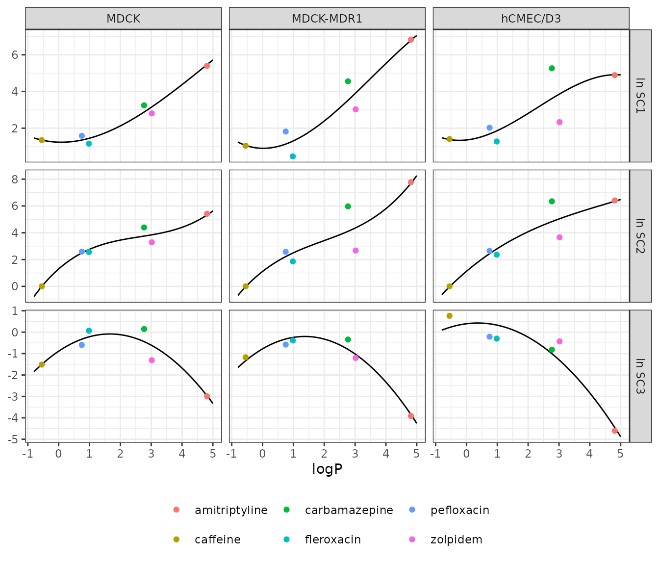

Replicates Figure 3 of Sanchez-Dengra 2021: ln(scaling factor) against logP with the printed QSPR polynomials.

Replicating Figure 4: brain profiles predicted from logP

In the paper’s internal validation, the fitted scaling factors of each model were replaced by those predicted from logP by the QSPR, and the brain profiles re-simulated (Figure 4). The packaged models do this with ini():

fig4 <- lapply(seq_len(nrow(grid)), function(i) {
  d <- design[design$drug == grid$drug[i], ]
  rows <- qspr[qspr$cell == grid$cell[i], ]
  sc_pred <- vapply(split(rows, rows$sc), function(r) qspr_predict(r, logp[[grid$drug[i]]]), numeric(1))
  m_qspr <- rxode2::ini(mods[[grid$model[i]]], sc1 = sc_pred[["sc1"]], sc2 = sc_pred[["sc2"]], sc3 = sc_pred[["sc3"]])
  obs <- sort(unique(c(seq(0, d$t_end, length.out = 401), 1:120)))
  obs <- obs[obs <= d$t_end]
  s_fit <- solve_one(grid$model[i], grid$drug[i], obs)
  s_qspr <- as.data.frame(rxode2::rxSolve(m_qspr, make_events(grid$drug[i], obs)))
  rbind(
    data.frame(drug = grid$drug[i], cell = grid$cell_label[i], scaling = "fitted (Table 3)", time = s_fit$time, brain = s_fit[[d$brain_var]]),
    data.frame(drug = grid$drug[i], cell = grid$cell_label[i], scaling = "QSPR (Figure 3)", time = s_qspr$time, brain = s_qspr[[d$brain_var]])
  )
})
#> ℹ change initial estimate of `sc1` to `235.653904194412`
#> ℹ change initial estimate of `sc2` to `205.200649808563`
#> ℹ change initial estimate of `sc3` to `0.0513374332458645`
#> ℹ change initial estimate of `sc1` to `883.810608583178`
#> ℹ change initial estimate of `sc2` to `2189.32466476364`
#> ℹ change initial estimate of `sc3` to `0.0213804398635012`
#> ℹ change initial estimate of `sc1` to `136.197051476877`
#> ℹ change initial estimate of `sc2` to `571.649087654199`
#> ℹ change initial estimate of `sc3` to `0.0116224500744908`
#> ℹ change initial estimate of `sc1` to `3.8669694986738`
#> ℹ change initial estimate of `sc2` to `0.987395115499673`
#> ℹ change initial estimate of `sc3` to `0.221379357340252`
#> ℹ change initial estimate of `sc1` to `2.89647795321618`
#> ℹ change initial estimate of `sc2` to `0.968381531740523`
#> ℹ change initial estimate of `sc3` to `0.262797895603704`
#> ℹ change initial estimate of `sc1` to `3.9784831358289`
#> ℹ change initial estimate of `sc2` to `0.968685772371473`
#> ℹ change initial estimate of `sc3` to `1.24642879699081`
#> ℹ change initial estimate of `sc1` to `17.8021435285496`
#> ℹ change initial estimate of `sc2` to `42.5511822673498`
#> ℹ change initial estimate of `sc3` to `0.642605739921859`
#> ℹ change initial estimate of `sc1` to `33.7401980841461`
#> ℹ change initial estimate of `sc2` to `60.64767130365`
#> ℹ change initial estimate of `sc3` to `0.447368249115635`
#> ℹ change initial estimate of `sc1` to `37.1296441778978`
#> ℹ change initial estimate of `sc2` to `125.267463576745`
#> ℹ change initial estimate of `sc3` to `0.366921885364807`
#> ℹ change initial estimate of `sc1` to `4.24113512680616`
#> ℹ change initial estimate of `sc2` to `15.5789923112935`
#> ℹ change initial estimate of `sc3` to `0.802666153940649`
#> ℹ change initial estimate of `sc1` to `3.64506993560694`
#> ℹ change initial estimate of `sc2` to `11.9838958502066`
#> ℹ change initial estimate of `sc3` to `0.780607200471536`
#> ℹ change initial estimate of `sc1` to `6.3694074291132`
#> ℹ change initial estimate of `sc2` to `16.2289038380435`
#> ℹ change initial estimate of `sc3` to `1.39540012206541`
#> ℹ change initial estimate of `sc1` to `3.86798761239766`
#> ℹ change initial estimate of `sc2` to `12.077871782013`
#> ℹ change initial estimate of `sc3` to `0.721489466731154`
#> ℹ change initial estimate of `sc1` to `3.10748121707528`
#> ℹ change initial estimate of `sc2` to `9.22590810824632`
#> ℹ change initial estimate of `sc3` to `0.72669385313198`
#> ℹ change initial estimate of `sc1` to `5.4007988348017`
#> ℹ change initial estimate of `sc2` to `11.452980479345`
#> ℹ change initial estimate of `sc3` to `1.47707310806705`
#> ℹ change initial estimate of `sc1` to `23.5448013823868`
#> ℹ change initial estimate of `sc2` to `46.8034369813749`
#> ℹ change initial estimate of `sc3` to `0.537032642254208`
#> ℹ change initial estimate of `sc1` to `50.2630014099727`
#> ℹ change initial estimate of `sc2` to `78.9839181482007`
#> ℹ change initial estimate of `sc3` to `0.353736426881636`
#> ℹ change initial estimate of `sc1` to `47.6810269068001`
#> ℹ change initial estimate of `sc2` to `155.194964191038`
#> ℹ change initial estimate of `sc3` to `0.268437061589189`
fig4 <- do.call(rbind, fig4)

ggplot(fig4, aes(time, brain, colour = cell, linetype = scaling)) +
  geom_line() +
  scale_linetype_manual(values = c("fitted (Table 3)" = "dashed", "QSPR (Figure 3)" = "solid")) +
  facet_wrap(~drug, scales = "free", ncol = 2) +
  labs(x = "t (s)", y = "Brain C (ng/mL)", colour = "Cell line", linetype = NULL) +
  theme_bw() +
  theme(legend.position = "bottom", legend.box = "vertical")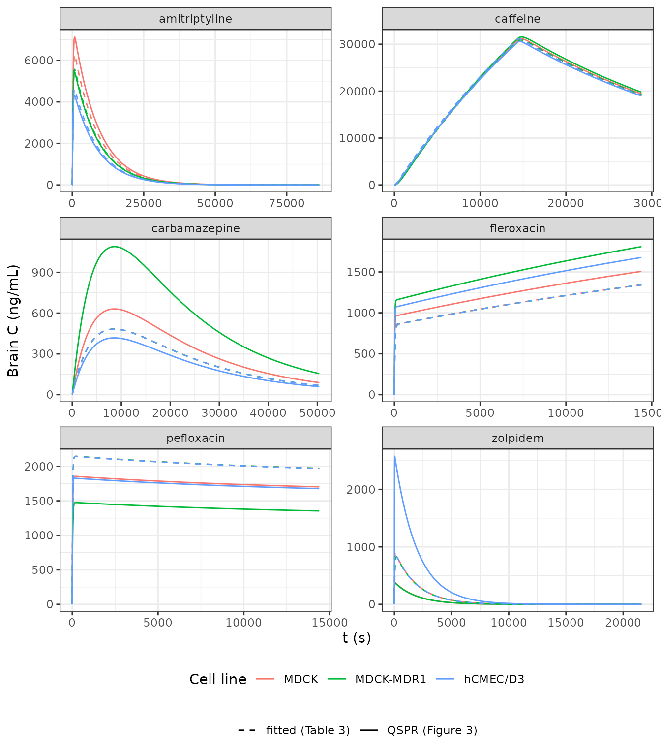

Replicates Figure 4 of Sanchez-Dengra 2021: brain profiles simulated with QSPR-predicted scaling factors (solid) against the fitted profiles (dashed).

The QSPR-predicted lines of Figure 4 were read by eye at their peaks (at the end of the record for fleroxacin, whose brain concentration rises throughout):

fig4_anchor <- data.frame(
  drug = rep(drugs, each = 3),
  cell = rep(unname(cells), times = 6),
  what = rep(c("peak", "peak", "peak", "end", "peak", "peak"), each = 3),
  figure4 = c(6300, 5500, 4000, 31000, 31000, 31000, 610, 1090, 410, 1500, 1800, 1680, 1850, 1480, 1840, 400, 380, 2550)
)
fig4_at <- function(drug, cell, what) {
  x <- fig4[fig4$drug == drug & fig4$cell == cell & fig4$scaling == "QSPR (Figure 3)", ]
  if (nrow(x) == 0L) stop("no simulated rows for ", drug, " ", cell)
  if (what == "peak") max(x$brain) else x$brain[which.max(x$time)]
}
fig4_anchor$simulated <- signif(mapply(fig4_at, fig4_anchor$drug, fig4_anchor$cell, fig4_anchor$what), 4)
fig4_anchor$pct_diff <- round(100 * (fig4_anchor$simulated / fig4_anchor$figure4 - 1), 1)
knitr::kable(fig4_anchor)

drug	cell	what	figure4	simulated	pct_diff
amitriptyline	MDCK	peak	6300	7125.0	13.1
amitriptyline	MDCK-MDR1	peak	5500	5428.0	-1.3
amitriptyline	hCMEC/D3	peak	4000	4301.0	7.5
caffeine	MDCK	peak	31000	31210.0	0.7
caffeine	MDCK-MDR1	peak	31000	31550.0	1.8
caffeine	hCMEC/D3	peak	31000	30610.0	-1.3
carbamazepine	MDCK	peak	610	630.8	3.4
carbamazepine	MDCK-MDR1	peak	1090	1089.0	-0.1
carbamazepine	hCMEC/D3	peak	410	417.7	1.9
fleroxacin	MDCK	end	1500	1507.0	0.5
fleroxacin	MDCK-MDR1	end	1800	1810.0	0.6
fleroxacin	hCMEC/D3	end	1680	1677.0	-0.2
pefloxacin	MDCK	peak	1850	1855.0	0.3
pefloxacin	MDCK-MDR1	peak	1480	1475.0	-0.3
pefloxacin	hCMEC/D3	peak	1840	1828.0	-0.7
zolpidem	MDCK	peak	400	381.5	-4.6
zolpidem	MDCK-MDR1	peak	380	372.8	-1.9
zolpidem	hCMEC/D3	peak	2550	2576.0	1.0

# Measured within 8 percent everywhere except amitriptyline/MDCK (+13
# percent, discussed below). A wrong QSPR coefficient or logP moves these
# predictions by tens of percent or more (compare the cell lines).
stopifnot(nrow(fig4_anchor) == 18L, all(abs(fig4_anchor$pct_diff) < 15))

The QSPR predictions reproduce Figure 4, including the two failures the paper discusses: carbamazepine is over-predicted with MDCK-MDR1 inputs and zolpidem with hCMEC/D3 inputs. The largest difference is the amitriptyline MDCK peak, 13 percent above the paper’s line. Two things plausibly contribute. The paper’s simulated lines are drawn through a few time points (the kinks in Figure 2A), which cuts off the top of a peak that lasts only minutes. And at logP = 4.81 the cubic term multiplies coefficient rounding by more than 100.

Brain exposure with PKNCA

Brain Cmax and AUC(0-tlast) of the fitted and QSPR-predicted profiles, by drug, cell line and scaling source:

conc_brain <- fig4 |>
  filter(!is.na(brain)) |>
  mutate(
    treatment = paste(drug, cell, scaling, sep = " | "),
    id = 1L,
    brain = pmax(brain, 0)
  )
dose_brain <- conc_brain |>
  distinct(treatment, id, drug) |>
  left_join(design |> mutate(total_dose = bolus_amt + inf_rate * inf_dur) |> select(drug, total_dose), by = "drug") |>
  mutate(time = 0)
o_conc_b <- PKNCAconc(conc_brain, brain ~ time | treatment + id)
o_dose_b <- PKNCAdose(dose_brain, total_dose ~ time | treatment + id)
o_data_b <- PKNCAdata(o_conc_b, o_dose_b,
  intervals = data.frame(start = 0, end = Inf, cmax = TRUE, auclast = TRUE)
)
nca_brain <- as.data.frame(pk.nca(o_data_b)) |>
  filter(PPTESTCD %in% c("cmax", "auclast")) |>
  select(treatment, PPTESTCD, PPORRES) |>
  pivot_wider(names_from = PPTESTCD, values_from = PPORRES) |>
  tidyr::separate(treatment, into = c("drug", "cell", "scaling"), sep = " \\| ")
stopifnot(nrow(nca_brain) == 36L, all(is.finite(nca_brain$cmax)), all(is.finite(nca_brain$auclast)))
knitr::kable(
  nca_brain |>
    dplyr::rename("Brain Cmax (ng/mL)" = cmax, "Brain AUC0-tlast (ng*s/mL)" = auclast),
  digits = 1
)

drug	cell	scaling	Brain AUC0-tlast (ng*s/mL)	Brain Cmax (ng/mL)
amitriptyline	hCMEC/D3	fitted (Table 3)	42752073.3	4596.5
amitriptyline	hCMEC/D3	QSPR (Figure 3)	40006743.3	4301.3
amitriptyline	MDCK	fitted (Table 3)	58238769.0	6255.2
amitriptyline	MDCK	QSPR (Figure 3)	66378937.6	7124.8
amitriptyline	MDCK-MDR1	fitted (Table 3)	51794361.5	5566.6
amitriptyline	MDCK-MDR1	QSPR (Figure 3)	50507299.0	5428.2
caffeine	hCMEC/D3	fitted (Table 3)	596509221.2	31180.9
caffeine	hCMEC/D3	QSPR (Figure 3)	586527354.3	30613.9
caffeine	MDCK	fitted (Table 3)	591949574.1	30935.2
caffeine	MDCK	QSPR (Figure 3)	597223844.1	31210.6
caffeine	MDCK-MDR1	fitted (Table 3)	591514195.7	30913.5
caffeine	MDCK-MDR1	QSPR (Figure 3)	604019387.8	31551.7
carbamazepine	hCMEC/D3	fitted (Table 3)	12977191.3	482.5
carbamazepine	hCMEC/D3	QSPR (Figure 3)	11234382.8	417.7
carbamazepine	MDCK	fitted (Table 3)	12981442.1	483.0
carbamazepine	MDCK	QSPR (Figure 3)	16958158.7	630.8
carbamazepine	MDCK-MDR1	fitted (Table 3)	12978295.7	482.6
carbamazepine	MDCK-MDR1	QSPR (Figure 3)	29357561.0	1089.4
fleroxacin	hCMEC/D3	fitted (Table 3)	16001196.6	1341.7
fleroxacin	hCMEC/D3	QSPR (Figure 3)	20031591.5	1677.1
fleroxacin	MDCK	fitted (Table 3)	16037841.8	1343.0
fleroxacin	MDCK	QSPR (Figure 3)	17994887.8	1507.2
fleroxacin	MDCK-MDR1	fitted (Table 3)	16002179.3	1341.8
fleroxacin	MDCK-MDR1	QSPR (Figure 3)	21605104.8	1809.6
pefloxacin	hCMEC/D3	fitted (Table 3)	29384508.7	2143.7
pefloxacin	hCMEC/D3	QSPR (Figure 3)	25055183.0	1828.4
pefloxacin	MDCK	fitted (Table 3)	29409257.0	2145.5
pefloxacin	MDCK	QSPR (Figure 3)	25426071.5	1855.2
pefloxacin	MDCK-MDR1	fitted (Table 3)	29419652.8	2146.3
pefloxacin	MDCK-MDR1	QSPR (Figure 3)	20212689.4	1475.0
zolpidem	hCMEC/D3	fitted (Table 3)	1805033.4	901.3
zolpidem	hCMEC/D3	QSPR (Figure 3)	5142535.5	2576.3
zolpidem	MDCK	fitted (Table 3)	1809477.4	873.7
zolpidem	MDCK	QSPR (Figure 3)	761744.7	381.5
zolpidem	MDCK-MDR1	fitted (Table 3)	1773751.9	825.3
zolpidem	MDCK-MDR1	QSPR (Figure 3)	745663.5	372.8

The paper does not tabulate brain Cmax or AUC. Its Table 4 gives the mean prediction error of the QSPR-simulated brain Cmax and AUC against the experimental data; those data are not published in tabular form, so Table 4 cannot be recomputed here. As a proxy, the prediction error of the QSPR-simulated profile against the fitted profile (which tracked the data with a mean AUC error near 5 percent, Table 4 first row) is:

pe <- nca_brain |>
  pivot_wider(names_from = scaling, values_from = c(cmax, auclast)) |>
  mutate(
    pe_cmax = 100 * abs(`cmax_fitted (Table 3)` - `cmax_QSPR (Figure 3)`) / `cmax_fitted (Table 3)`,
    pe_auc = 100 * abs(`auclast_fitted (Table 3)` - `auclast_QSPR (Figure 3)`) / `auclast_fitted (Table 3)`
  )
pe_summary <- pe |>
  group_by(cell) |>
  summarise(mean_pe_cmax = mean(pe_cmax), mean_pe_auc = mean(pe_auc), .groups = "drop") |>
  mutate(cell = factor(cell, levels = cells)) |>
  arrange(cell) |>
  mutate(
    paper_pe_cmax = c(19.23, 35.71, 49.77),
    paper_pe_auc = c(22.34, 48.21, 46.69)
  )
knitr::kable(
  pe_summary |>
    dplyr::rename(
      "Cell line" = cell,
      "Mean PE% Cmax (QSPR vs fitted)" = mean_pe_cmax,
      "Mean PE% AUC (QSPR vs fitted)" = mean_pe_auc,
      "Table 4 PE% Cmax (vs data)" = paper_pe_cmax,
      "Table 4 PE% AUC (vs data)" = paper_pe_auc
    ),
  digits = 1
)

Cell line	Mean PE% Cmax (QSPR vs fitted)	Mean PE% AUC (QSPR vs fitted)	Table 4 PE% Cmax (vs data)	Table 4 PE% AUC (vs data)
MDCK	21.2	21.5	19.2	22.3
MDCK-MDR1	41.9	42.5	35.7	48.2
hCMEC/D3	41.2	41.1	49.8	46.7

# The paper's conclusion (MDCK predicts best) holds for the proxy too:
# measured 21.5 percent AUC error for MDCK against 42.5 and 41.1.
stopifnot(nrow(pe_summary) == 3L, which.min(pe_summary$mean_pe_auc) == 1L, which.min(pe_summary$mean_pe_cmax) == 1L)

The proxy and Table 4 measure different things – the proxy excludes the fitting error and the paper’s PE% is taken as a signed per-drug value before averaging (Equation 15) – so the numbers are shown side by side rather than compared. The paper’s conclusion that the MDCK-based QSPR gives the best predictions is visible in both.

Assumptions and deviations

• Eighteen files for one structure. The paper fitted each drug separately for each of the three cell lines (Table 3), so each drug-cell-line combination is its own model, named SanchezDengra_2021_<drug>_rat_pbpk_<cellline>. The in vivo parameters Vd, kel and ka are the same in the three files of a drug because Table 3 reports a single value per drug.
• Deterministic model. No between-animal variability or residual error was estimated (mean profiles fitted in Berkeley Madonna), so the models have no eta or residual-error terms.
• Time in seconds. All rate constants, flows and infusion rates are printed per second; the models keep the paper’s units (time s, dose ng, concentration ng/mL, volume cm^3 = mL).
• Physiological flows used as printed. Qbulk = 0.012 cm^3/s and Qsink = 0.132 cm^3/s (Methods 2.4, citing Ball et al.) are large compared with the rat brain interstitial and CSF flows used elsewhere in this package (0.2 and 2.2 uL/min in Yamamoto_2017_quinidine_rat_pbpk, Table 3 of that paper). They are used exactly as printed, because the fitted scaling factors were estimated with them and the Figure 2 fits are reproduced with them (see the anchor check above); any unit inconsistency in the physiological constants is absorbed by the fitted SC1-SC3.
• Rounded amitriptyline SC3. Table 3 prints amitriptyline’s SC3 as 0.05 (MDCK), 0.02 (MDCK-MDR1) and 0.01 (hCMEC/D3). The models use these printed values. As a result the MDCK-MDR1 and hCMEC/D3 total brain concentrations of amitriptyline are 11 and 27 percent lower than the MDCK ones, whereas the paper’s fits overlap. Unbound brain concentrations are not affected. The unrounded values implied by the overlap and by Figure 3 are about 0.018 and 0.0073.
• Caffeine infusion duration. Table 1 gives the caffeine infusion rate (833.333 ng/s) but not its duration; 14,400 s (4 h) was taken from the peak of the fitted lines in Figure 2B.
• Fleroxacin and pefloxacin dosing. Table 1 gives both D and k0; D is modelled as an intravenous bolus at time zero followed by the infusion for the whole record, which reproduces the non-zero starting plasma concentrations of Figure 2D-E.
• Extravascular route and bioavailability. Equations 7-8 feed the whole dose through ka into plasma; bioavailability is not a parameter, so any incomplete absorption is absorbed into the fitted Vd.
• kel and ka source trace. The values are copied from Table 3, where they are printed in x 10^-n notation (for example amitriptyline kel = 1.17 x 10^-4 s^-1).
• Errata. No erratum or correction was found for this article (Crossref update metadata, checked 2026-09-29).