Sacituzumab govitecan exposure-response in mTNBC (Sathe 2025b)
Source:vignettes/articles/Sathe_2025b_sacituzumab_exposure_response.Rmd
Sathe_2025b_sacituzumab_exposure_response.RmdSource and models
Sathe AG, Diderichsen PM, Fauchet F, Phan SC, Girish S, Othman AA. Exposure-Response Analyses of Sacituzumab Govitecan Efficacy and Safety in Patients With Metastatic Triple-Negative Breast Cancer. Clin Pharmacol Ther 2025;117(2):570-578. doi:10.1002/cpt.3495.
The paper relates individual exposure of sacituzumab govitecan (SG,
an anti-Trop-2 antibody-drug conjugate carrying SN-38) to efficacy and
safety in 277 patients with metastatic triple-negative breast cancer.
Exposures come from the companion population PK model of Sathe 2024,
packaged as Sathe_2024_sacituzumab. The b in
the file stem separates this paper from
Sathe_2025_sacituzumab, an unrelated 2025 update of that
population PK model.
Six models are packaged, one per endpoint the paper fitted with reported coefficients:
| Model | Endpoint | Form | Exposure driver |
|---|---|---|---|
Sathe_2025b_sacituzumab_cr |
Complete response (BICR) | logistic | CAVG of intact SG |
Sathe_2025b_sacituzumab_orr |
Objective response (BICR) | logistic | CAVG of intact SG |
Sathe_2025b_sacituzumab_pfs |
Progression-free survival | Cox PH + 12-month landmark | CAVG of total antibody |
Sathe_2025b_sacituzumab_os |
Overall survival | Cox PH + 12-month landmark | CAVG of total antibody |
Sathe_2025b_sacituzumab_diarrhea |
Worst diarrhea grade (>= 1, >= 3) | nonproportional-odds logistic | CAVG of intact SG |
Sathe_2025b_sacituzumab_neutropenia |
Worst neutropenia grade (>= 1, >= 3, 4) | nonproportional-odds logistic | CAVG of intact SG |
None of the models has a PK layer, a random effect or an ODE: each is
a deterministic function of per-patient covariates, with exposure
supplied as the CAV data column.
mod_cr   <- readModelDb("Sathe_2025b_sacituzumab_cr")
mod_orr  <- readModelDb("Sathe_2025b_sacituzumab_orr")
mod_pfs  <- readModelDb("Sathe_2025b_sacituzumab_pfs")
mod_os   <- readModelDb("Sathe_2025b_sacituzumab_os")
mod_diar <- readModelDb("Sathe_2025b_sacituzumab_diarrhea")
mod_neut <- readModelDb("Sathe_2025b_sacituzumab_neutropenia")

# One solve per covariate row; no dosing, no time course.
solve_er <- function(model, covs) {
  ev <- data.frame(id = seq_len(nrow(covs)), time = 0, amt = 0, evid = 0L, covs)
  as.data.frame(suppressWarnings(
    rxode2::rxSolve(model, events = ev, returnType = "data.frame")
  ))
}
Exposure metric
The exposure for every endpoint is an average concentration from the
first dose to an endpoint-specific time t_event (Sathe
2025b Eq. 1 and Table S1):
computed from the population PK predictions with each patient’s
actual doses, reductions and delays. t_event is the first
response for CR and ORR, the first report of the worst adverse-event
grade for the safety endpoints, and the event or censoring time for PFS
and OS (in each case capped at 21 days after the last dose). The same
analyte therefore yields a different column for each endpoint: the mean
intact-SG CAVG at 10 mg/kg was 17.5 ug/mL for ORR, 22.1 ug/mL for
neutropenia and 29.7 ug/mL for diarrhea (Figure 1 and Figure 3
captions). Use the SG output Cc of
Sathe_2024_sacituzumab for the CR, ORR and safety models,
and its total-antibody output Cc_tab for PFS and OS.
Population
Pooled patients with metastatic triple-negative breast cancer from the phase I/II IMMU-132-01 study (n = 24) and the SG arm of the phase III ASCENT study (n = 253) who had population PK exposure estimates and at least one outcome (Sathe 2025b Results and Table S3). Median age 54 years (range 27-82), median body weight 66.7 kg (37.2-132), 99.3% female, 80.5% White, 67.9% from North America. Median baseline LDH 277 IU/L (107-5930). Prior therapy: platinum-based only 48.0%, checkpoint inhibitor only 9.0%, both 19.1%, neither (“Others”) 23.8%. Starting doses were 8 mg/kg (16 in IMMU-132-01 and 4 in ASCENT), 10 mg/kg (5 and 249) and 12 mg/kg (3 in IMMU-132-01), on days 1 and 8 of 21-day cycles. PFS was missing for two ASCENT patients (n = 275).
Source trace
| Quantity | Value | Source |
|---|---|---|
| CR intercept, slope per ug/mL CAVG_SG | -8.89, 0.309 | Table S7 |
| ORR intercept, slope per ug/mL CAVG_SG | -6.96, 0.343 | Table S7 |
| PFS log-HR per ug/mL CAVG_tAB | -0.00730 | Table S10 |
| PFS log-HR, prior CPI / platinum / both vs Others | 0.495 / 0.736 / 1.01 | Table S10 |
| PFS 12-month baseline cumulative hazard | 3.43 | back-solved from the 8 rows of Table S11 |
| OS log-HR per ug/mL CAVG_tAB, per IU/L LDH | -0.0123, 0.000622 | Table S10 |
| OS 12-month baseline cumulative hazard | 3.31 | back-solved from the median-LDH rows of Table S12 at LDH 277 IU/L (Table S3) |
| Diarrhea grade >= 1: odds ratio; intercept | 1.45; -6.52 | Table 3; digitised from Figure 3a |
| Diarrhea grade >= 3: odds ratio; intercept | 1.01; -2.40 | Table 3; approximated from Table 3 (0.109 at 10 mg/kg) and the Figure 3 caption mean CAVG_SG 29.7 ug/mL |
| Neutropenia grade >= 1: odds ratio; intercept | 1.37; -5.63 | Table 3; digitised from Figure 3b |
| Neutropenia grade >= 3: odds ratio; intercept | 1.09; -1.68 | Table 3; digitised from Figure 3c |
| Neutropenia grade 4: odds ratio; intercept | 1.03; -2.13 | Table 3; approximated from Table 3 (0.186 at 10 mg/kg) and the Figure 3 caption mean CAVG_SG 22.1 ug/mL |
Logistic link logit(p) = b0 + b * X
|
Supplementary Eq. 1 and Eq. 4 | |
Cox model h(t) = h0(t) exp(b * X),
S(t) = exp(-H(t))
|
Supplementary Eq. 2 and Eq. 3 |
Virtual cohort
The models carry no between-subject variability, so a stochastic cohort adds nothing: every prediction below is a deterministic function of the covariates on its row. The exposure values used are the ones the paper itself reports – the mean CAVG of the 8 and 10 mg/kg starting-dose groups (figure captions and Tables S11-S12) and the CAVG_tAB quartile medians of Table 2 – so each check is a like-for-like comparison with a printed number.
Efficacy: complete and objective response
grid_sg <- data.frame(CAV = seq(7, 30, by = 0.25))
resp <- bind_rows(
  solve_er(mod_cr, grid_sg) |> transmute(CAV, p = prob_cr_central, Endpoint = "(a) Complete response"),
  solve_er(mod_orr, grid_sg) |> transmute(CAV, p = prob_orr_central, Endpoint = "(b) Objective response")
)
ggplot(resp, aes(CAV, p)) +
  geom_line(linewidth = 0.8) +
  facet_wrap(~Endpoint) +
  scale_y_continuous(limits = c(0, 1)) +
  labs(x = "CAVG of intact SG (ug/mL)", y = "Probability") +
  theme_bw()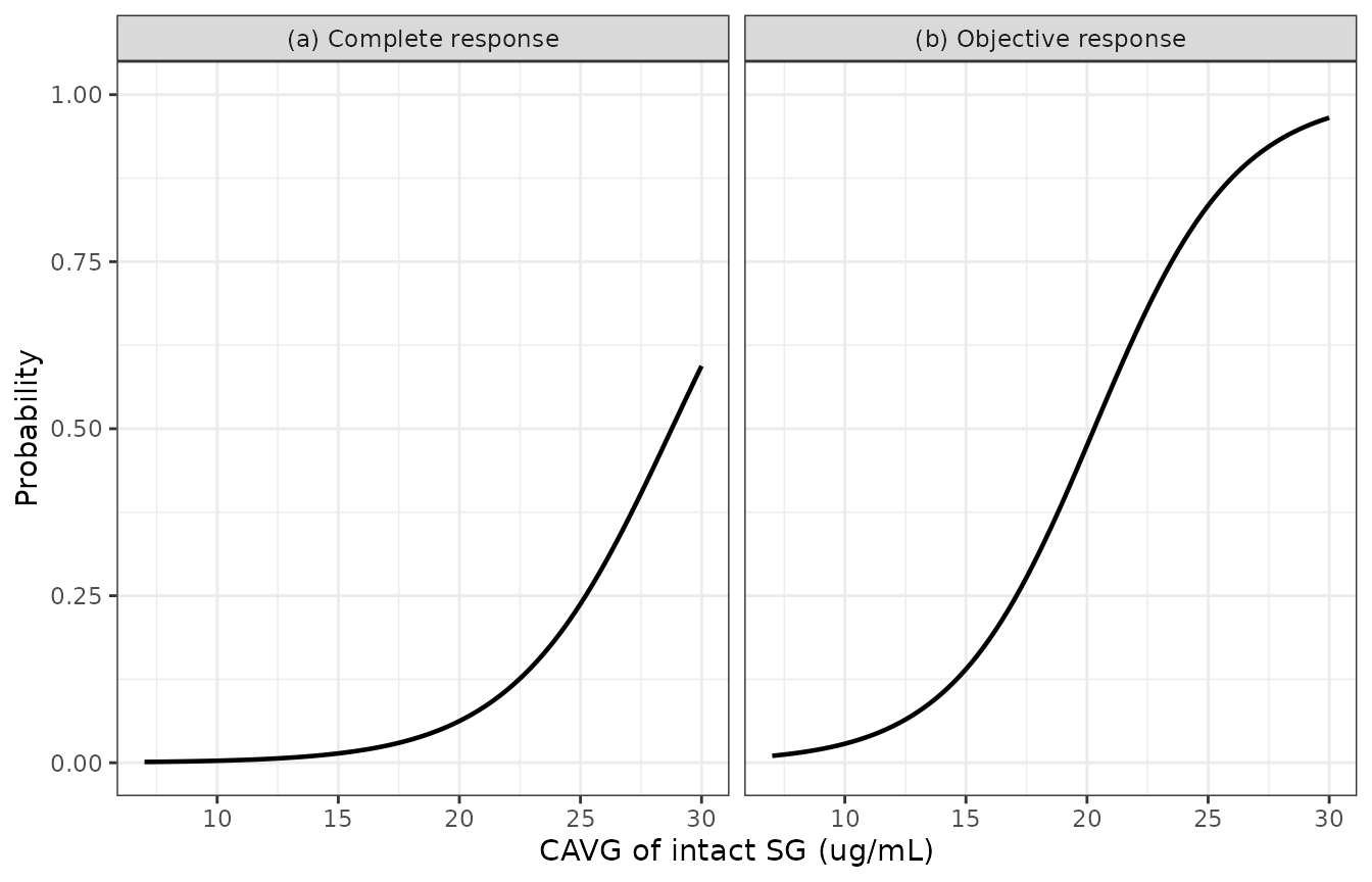
Replicates Figure 1 of Sathe 2025b: model-predicted probability of complete response (a) and objective response (b) against the average concentration of intact SG.
The printed predictions at 10 mg/kg (CR 4.26%, ORR 32.6%; Table 1) are averages over the 258 patients of that group, each at their own exposure, and equal the observed proportions – as they must for a maximum-likelihood logistic fit with an intercept. They are not the probability at the group’s mean exposure:
at_mean <- data.frame(CAV = c(12.6, 16.8, 12.9, 17.5))
p_mean <- c(
  solve_er(mod_cr, at_mean[1:2, , drop = FALSE])$prob_cr_central,
  solve_er(mod_orr, at_mean[3:4, , drop = FALSE])$prob_orr_central
)
data.frame(
  Endpoint = c("CR", "CR", "ORR", "ORR"),
  `Starting dose` = c("8 mg/kg", "10 mg/kg", "8 mg/kg", "10 mg/kg"),
  `Mean CAVG_SG (ug/mL)` = at_mean$CAV,
  `Probability at mean CAVG` = signif(p_mean, 3),
  `Table 1 dataset prediction` = c(0, 0.0426, 0.125, 0.326),
  check.names = FALSE
) |> knitr::kable()| Endpoint | Starting dose | Mean CAVG_SG (ug/mL) | Probability at mean CAVG | Table 1 dataset prediction |
|---|---|---|---|---|
| CR | 8 mg/kg | 12.6 | 0.00672 | 0.0000 |
| CR | 10 mg/kg | 16.8 | 0.02420 | 0.0426 |
| ORR | 8 mg/kg | 12.9 | 0.07340 | 0.1250 |
| ORR | 10 mg/kg | 17.5 | 0.27700 | 0.3260 |
At 10 mg/kg the probability at the mean exposure (0.277) sits below the dataset average of 0.326 because the logistic curve is convex over most of the exposure range, so averaging over the exposure spread raises the mean probability.
Efficacy: progression-free and overall survival
Both Cox models return the relative hazard hr and a
12-month landmark probability exp(-H0(12) * hr). The
baseline cumulative hazard is not printed; it was back-solved from the
paper’s own predictions, so the strongest available check is that the
eight PFS rows of Table S11, which share a single H0(12),
are all reproduced at once.
s11 <- data.frame(
  Category = rep(c("CPI", "Platinum based", "CPI + platinum based", "Others"), each = 2),
  Dose = rep(c("8 mg/kg", "10 mg/kg"), 4),
  CAV = rep(c(122, 152), 4),
  PRIOR_CHECKPOINT_INHIBITOR = rep(c(1, 0, 1, 0), each = 2),
  PRIOR_PLATIN = rep(c(0, 1, 1, 0), each = 2),
  published = c(0.0991, 0.156, 0.0528, 0.0938, 0.0212, 0.0450, 0.244, 0.322)
)
s11$model <- solve_er(mod_pfs, s11[, c("CAV", "PRIOR_CHECKPOINT_INHIBITOR", "PRIOR_PLATIN")])$prob_pfs_12mo
s11 |>
  transmute(
    `Prior treatment` = Category, `Starting dose` = Dose, `Mean CAVG_tAB` = CAV,
    `Table S11` = published, `Model` = signif(model, 3),
    `Difference` = signif(model - published, 2)
  ) |>
knitr::kable()| Prior treatment | Starting dose | Mean CAVG_tAB | Table S11 | Model | Difference |
|---|---|---|---|---|---|
| CPI | 8 mg/kg | 122 | 0.0991 | 0.0993 | 0.00023 |
| CPI | 10 mg/kg | 152 | 0.1560 | 0.1560 | 0.00043 |
| Platinum based | 8 mg/kg | 122 | 0.0528 | 0.0529 | 0.00014 |
| Platinum based | 10 mg/kg | 152 | 0.0938 | 0.0944 | 0.00055 |
| CPI + platinum based | 8 mg/kg | 122 | 0.0212 | 0.0210 | -0.00024 |
| CPI + platinum based | 10 mg/kg | 152 | 0.0450 | 0.0448 | -0.00017 |
| Others | 8 mg/kg | 122 | 0.2440 | 0.2450 | 0.00070 |
| Others | 10 mg/kg | 152 | 0.3220 | 0.3230 | 0.00076 |
For OS, Table S12 gives predictions at the lower quartile, median and upper quartile of LDH, but the paper prints only the median (277 IU/L, Table S3). The baseline cumulative hazard was back-solved from the two median rows; the other four rows then reveal the LDH quartiles the authors used.
s12 <- data.frame(
  LDH_level = rep(c("Lower quartile", "Median", "Upper quartile"), each = 2),
  CAV = rep(c(125, 148), 3),
  published = c(0.446, 0.546, 0.429, 0.530, 0.390, 0.494)
)
ini_os <- rxode2::rxode(mod_os)$theta
H0_os <- ini_os[["ch0_os_12mo"]]
s12$implied_LDH <- (log(-log(s12$published) / H0_os) - ini_os[["e_cav_os_haz"]] * s12$CAV) /
  ini_os[["e_ldh_os_haz"]]
med <- s12$LDH_level == "Median"
s12$model <- NA_real_
s12$model[med] <- solve_er(mod_os, data.frame(CAV = s12$CAV[med], LDH = 277))$prob_os_12mo
s12 |>
  transmute(
    `LDH level` = LDH_level, `Mean CAVG_tAB` = CAV, `Table S12` = published,
    `Model at LDH 277` = signif(model, 3), `Implied LDH (IU/L)` = round(implied_LDH)
  ) |>
knitr::kable()| LDH level | Mean CAVG_tAB | Table S12 | Model at LDH 277 | Implied LDH (IU/L) |
|---|---|---|---|---|
| Lower quartile | 125 | 0.446 | NA | 204 |
| Lower quartile | 148 | 0.546 | NA | 195 |
| Median | 125 | 0.429 | 0.429 | 279 |
| Median | 148 | 0.530 | 0.529 | 272 |
| Upper quartile | 125 | 0.390 | NA | 451 |
| Upper quartile | 148 | 0.494 | NA | 441 |
The implied quartiles, about 200 and 446 IU/L, bracket the 277 IU/L median asymmetrically, as expected for the right-skewed LDH distribution (range up to 5930 IU/L). Each quartile is implied consistently by the 8 and 10 mg/kg rows (within 10 IU/L), which confirms that the exposure slope and the 8 and 10 mg/kg mean exposures were read correctly.
q_pfs <- c(95.1, 130, 158, 205)
q_os <- c(88.7, 125, 153, 204)
pfs_grid <- expand.grid(
  CAV = q_pfs, cat = c("Others", "CPI", "Platinum based", "CPI + platinum based"),
  stringsAsFactors = FALSE
)
pfs_grid$PRIOR_CHECKPOINT_INHIBITOR <- as.numeric(grepl("CPI", pfs_grid$cat))
pfs_grid$PRIOR_PLATIN <- as.numeric(grepl("latinum", pfs_grid$cat))
pfs_grid$p <- solve_er(mod_pfs, pfs_grid[, c("CAV", "PRIOR_CHECKPOINT_INHIBITOR", "PRIOR_PLATIN")])$prob_pfs_12mo
os_grid <- data.frame(CAV = q_os, LDH = 277)
os_grid$p <- solve_er(mod_os, os_grid)$prob_os_12mo
bind_rows(
  pfs_grid |> transmute(CAV, p, Curve = paste("PFS:", cat), Endpoint = "PFS at 12 months"),
  os_grid |> transmute(CAV, p, Curve = "OS: median LDH", Endpoint = "OS at 12 months")
) |>
  ggplot(aes(CAV, p, colour = Curve)) +
  geom_line() + geom_point() +
  facet_wrap(~Endpoint) +
  labs(x = "CAVG of total antibody, quartile median (ug/mL)", y = "Probability", colour = NULL) +
  theme_bw()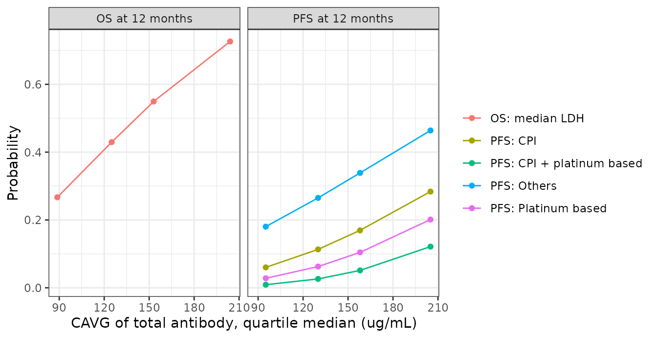
Typical 12-month landmark probabilities across the CAVG_tAB quartile medians of Table 2. PFS is shown per prior-treatment category; OS at the median LDH of 277 IU/L.
Safety: diarrhea and neutropenia
The adverse-event models are nonproportional-odds logistic regressions of the worst grade: each cumulative threshold has its own intercept and its own exposure slope (Supplementary Eq. 4). Table 3 prints the slopes as odds ratios but no intercept is printed anywhere. The intercepts for the three thresholds with a published fitted curve (Figure 3a-c) were recovered by digitising the solid curve with the slope held at the printed odds ratio; a free two-parameter fit to the same pixels returned odds ratios of 1.452, 1.376 and 1.093 against the printed 1.45, 1.37 and 1.09, which confirms the digitisation.
digitised <- tibble::tribble(
  ~Panel, ~CAV, ~p,
  "(a) Diarrhea grade >= 1", 11.68, 0.10,
  "(a) Diarrhea grade >= 1", 16.73, 0.40,
  "(a) Diarrhea grade >= 1", 17.83, 0.50,
  "(a) Diarrhea grade >= 1", 18.94, 0.60,
  "(a) Diarrhea grade >= 1", 23.99, 0.90,
  "(b) Neutropenia grade >= 1", 7.85, 0.041,
  "(b) Neutropenia grade >= 1", 10.00, 0.074,
  "(b) Neutropenia grade >= 1", 14.03, 0.225,
  "(b) Neutropenia grade >= 1", 17.96, 0.503,
  "(b) Neutropenia grade >= 1", 21.99, 0.783,
  "(b) Neutropenia grade >= 1", 26.11, 0.935,
  "(c) Neutropenia grade >= 3", 7.85, 0.257,
  "(c) Neutropenia grade >= 3", 15.82, 0.414,
  "(c) Neutropenia grade >= 3", 23.96, 0.594,
  "(c) Neutropenia grade >= 3", 32.01, 0.747,
  "(c) Neutropenia grade >= 3", 39.98, 0.856,
  "(c) Neutropenia grade >= 3", 49.91, 0.939
)
grid_ae <- data.frame(CAV = seq(5, 52, by = 0.25))
d_grid <- solve_er(mod_diar, grid_ae)
n_grid <- solve_er(mod_neut, grid_ae)
curves <- bind_rows(
  data.frame(Panel = "(a) Diarrhea grade >= 1", CAV = grid_ae$CAV, p = d_grid$prob_diarrhea),
  data.frame(Panel = "(b) Neutropenia grade >= 1", CAV = grid_ae$CAV, p = n_grid$prob_neutropenia),
  data.frame(Panel = "(c) Neutropenia grade >= 3", CAV = grid_ae$CAV, p = n_grid$prob_neutropenia_grade3)
)
ggplot(curves, aes(CAV, p)) +
  geom_line(linewidth = 0.8) +
  geom_point(data = digitised, colour = "firebrick") +
  facet_wrap(~Panel, scales = "free_x") +
  scale_y_continuous(limits = c(0, 1)) +
  labs(x = "CAVG of intact SG (ug/mL)", y = "Cumulative probability") +
  theme_bw()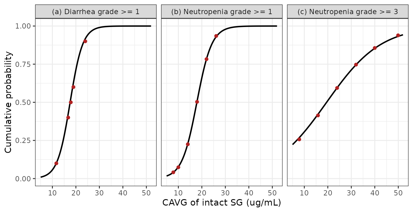
Replicates Figure 3 of Sathe 2025b: model curves with points read off the published fitted curves (not the observed quartile proportions).
dig_d <- digitised[digitised$Panel == "(a) Diarrhea grade >= 1", ]
dig_n1 <- digitised[digitised$Panel == "(b) Neutropenia grade >= 1", ]
dig_n3 <- digitised[digitised$Panel == "(c) Neutropenia grade >= 3", ]
resid <- c(
  solve_er(mod_diar, dig_d["CAV"])$prob_diarrhea - dig_d$p,
  solve_er(mod_neut, dig_n1["CAV"])$prob_neutropenia - dig_n1$p,
  solve_er(mod_neut, dig_n3["CAV"])$prob_neutropenia_grade3 - dig_n3$p
)
# Each point is read to about one pixel; the steep diarrhea panel has about
# 3 pixels per ug/mL, so its residuals are the largest.
stopifnot(max(abs(resid)) < 0.04)
The two thresholds that have no published curve (diarrhea grade >=
3 and neutropenia grade 4) had their intercepts approximated from the
Table 3 predicted proportion at 10 mg/kg, treated as the probability at
the Figure 3 caption’s mean exposure:
logit(p) - log(OR) * mean CAVG. The same shortcut can be
tested on neutropenia grade >= 3, where the digitised intercept is
available:
shortcut_n3 <- qlogis(0.543) - log(1.09) * 22.1
digitised_n3 <- rxode2::rxode(mod_neut)$theta[["neutropenia_grade3_intercept"]]
c(shortcut = round(shortcut_n3, 2), digitised = digitised_n3)
#>  shortcut digitised
#>     -1.73     -1.68
stopifnot(abs(shortcut_n3 - digitised_n3) < 0.15)
The shortcut lands within 0.05 logit units of the digitised value here, where the slope is shallow. Its error grows with the slope, which is why it was not used for the three steep thresholds that could be digitised instead.
The thresholds cross
Because each threshold has its own slope, the published cumulative curves are not ordered over the whole exposure range: the grade >= 3 neutropenia curve lies above the grade >= 1 curve below about 17 ug/mL (compare Figure 3b and 3c at 10 ug/mL: about 0.08 against 0.31). This is a property of the published model, not of the extraction. Read each output as its own threshold probability, and do not difference them to get per-grade probabilities in that range.
bind_rows(
  data.frame(CAV = grid_ae$CAV, p = n_grid$prob_neutropenia, Threshold = "grade >= 1", AE = "Neutropenia"),
  data.frame(CAV = grid_ae$CAV, p = n_grid$prob_neutropenia_grade3, Threshold = "grade >= 3", AE = "Neutropenia"),
  data.frame(CAV = grid_ae$CAV, p = n_grid$prob_neutropenia_grade4, Threshold = "grade 4", AE = "Neutropenia"),
  data.frame(CAV = grid_ae$CAV, p = d_grid$prob_diarrhea, Threshold = "grade >= 1", AE = "Diarrhea"),
  data.frame(CAV = grid_ae$CAV, p = d_grid$prob_diarrhea_grade3, Threshold = "grade >= 3", AE = "Diarrhea")
) |>
  ggplot(aes(CAV, p, linetype = Threshold)) +
  geom_line() +
  facet_wrap(~AE) +
  labs(x = "CAVG of intact SG (ug/mL)", y = "Cumulative probability") +
  theme_bw()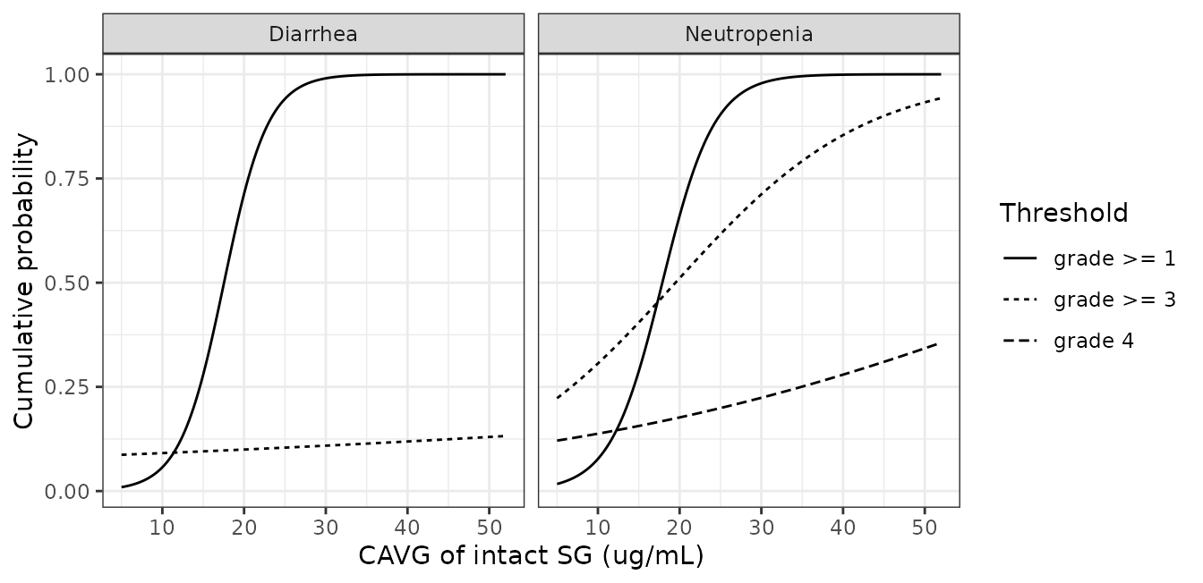
Cumulative threshold probabilities of the worst neutropenia and diarrhea grade.
PKNCA
Not applicable. None of the six models has a concentration-time
profile: the exposure is an input column, and the exposure-generating
population PK model is Sathe_2024_sacituzumab, whose own
vignette carries the NCA validation.
Assumptions and deviations
-
Intercepts of the adverse-event models are not
published. Three were digitised from Figure 3 with the slope
held at the printed odds ratio (uncertain by about one pixel: +/-0.2 on
the logit for the steep diarrhea panel, less for the others). Two –
diarrhea grade >= 3 and neutropenia grade 4 – have no curve and were
approximated from a dataset-averaged prediction treated as the
prediction at the mean exposure. Both slopes are non-significant and
printed to three significant figures, so
log(1.01)carries roughly +/-50% relative rounding uncertainty. Treat these two outputs as indicative. - Vomiting and nausea are not packaged. Table 3 gives their odds ratios, but no curve and no mean exposure are published for them, so neither the digitisation nor the approximation used for the other thresholds is possible.
- Time to first dose reduction and to first dose delay are not packaged. The paper reports only 12-month probabilities at the group-mean exposure (Table 4), with no coefficients and no mean exposure for those endpoints.
-
The 12-month baseline cumulative hazards are
back-solved, not printed. A Cox fit leaves
h0(t)nonparametric, soprob_pfs_12moandprob_os_12moare valid at 12 months only; the relative hazardhris valid at any time under proportional hazards. The paper notes that the proportional-hazards assumption was formally violated for CAVG_tAB but accepted after residual diagnostics. - Median LDH. The abstract quotes “median lactate dehydrogenase (227 IU/L)”; Table S3 gives 277 IU/L, with study medians of 241 and 283 IU/L. The pooled median must lie between the study medians, so 227 is a digit transposition and 277 was used to back-solve the OS baseline hazard.
-
Prior-treatment encoding. The paper’s four-level
factor is decomposed into
PRIOR_PLATINandPRIOR_CHECKPOINT_INHIBITOR, with the printed coefficient for the combined cell applied as is. The three coefficients are not additive (0.495 + 0.736 = 1.23 against 1.01). - Starting-dose group sizes. The Results text gives 20 patients at 8 mg/kg and 254 at 10 mg/kg; Table 1 and the Table S11-S12 footnotes use 16 and 258. The difference does not affect any coefficient; the means used here are the ones the tables print.
- Placeholder residual error. The source likelihoods are Bernoulli or multinomial with no residual; each probability output carries a fixed additive SD of 0.001 only so that the observation machinery accepts the model.