Erythroferrone in CKD and chemotherapy-induced anemia, rat (Zhang 2025)
Source:vignettes/articles/Zhang_2025_erythroferrone.Rmd
Zhang_2025_erythroferrone.Rmd
ckd_name <- "Zhang_2025_epoetinAlfa_erythroferrone_ckd_rat"
cia_name <- "Zhang_2025_epoetinAlfa_erythroferrone_cia_rat"

ckd <- rxode2::rxode(readModelDb(ckd_name))
cia <- rxode2::rxode(readModelDb(cia_name))
Model and source
Zhang 2025 develops two mechanism-based PK/PD models of erythroferrone (ERFE) in anemic rats – one per disease model – sharing an ERFE sub-model but differing in the erythroid-response structure and in every estimated parameter. Following the nlmixr2lib “replicate the author’s structure” policy they are packaged as two model files with this single validation vignette.
| Model file | Disease model | Erythroid structure | Drugs |
|---|---|---|---|
| Zhang_2025_epoetinAlfa_erythroferrone_ckd_rat | Adenine-induced CKD anemia (Figure 1A) | Lifespan-based indirect response, zero-order progenitor input
kIN0 stimulated by rHuEPO |
rHuEPO |
| Zhang_2025_epoetinAlfa_erythroferrone_cia_rat | Carboplatin-induced anemia (Figure 1B) | Friberg-Karlsson self-renewing progenitor pool inhibited by carboplatin | rHuEPO + carboplatin |
- Citation: Zhang L, Xu P, Yan X. Mechanism-Based Pharmacokinetic/Pharmacodynamic Modeling of Erythroferrone in Anemic Rats with Chronic Kidney Disease and Chemotherapy-Induced Anemia: An Early Biomarker for Hemoglobin Response and rHuEPO Hyporesponsiveness. ACS Pharmacol Transl Sci. 2025;8(1):189-202. doi:10.1021/acsptsci.4c00575. rHuEPO PK parameters fixed from Fan X, Krzyzanski W, Wong RSM, Yan X. J Pharmacol Exp Ther. 2022;382(1):31-43, as tabulated in Zhang 2025 Supporting Information Table S1.
- Article: https://doi.org/10.1021/acsptsci.4c00575
- Supplement (open access): https://doi.org/10.1021/acsptsci.4c00575 (“Supporting
Information”,
pt4c00575_si_001.pdf; contains Table S1 with the fixed PK parameters and Figures S1-S6)
CKD model description:
Preclinical (rat). Mechanism-based PK/PD model of erythroferrone (ERFE), hemoglobin and red blood cells after intravenous recombinant human erythropoietin (rHuEPO / epoetin alfa) in adenine-induced chronic-kidney-disease anemic rats (Zhang 2025, model structure of Figure 1A). rHuEPO PK is a two-compartment model with parallel linear and Michaelis-Menten elimination, fixed from prior rat studies (Table S1). The erythroid response is a lifespan-based indirect-response chain: a zero-order progenitor input kIN0, linearly stimulated by rHuEPO concentration and damped by an (RBC0 / RBC)^gamma feedback, feeds BFU-E (precursor1) which amplifies AMPN-fold into CFU-E (precursor2), amplifies AMPC-fold into erythroblasts (precursor3), then reticulocytes (precursor4) and circulating erythrocytes; hemoglobin is derived algebraically from the RBC count and the mean corpuscular hemoglobin. Circulating ERFE receives two simultaneous inputs: a circadian baseline pool driven by a cosinor production rate kCINE (mesor RM, amplitude RA, acrophase tpeak), and an rHuEPO-stimulated pool whose production is proportional to the erythroblast mass (precursor3) and to an Emax / EC50 function of rHuEPO concentration, delayed by two transit compartments. Fitted in NONMEM 7.5 with interindividual variability fixed to zero, so the model is a typical-value mechanism with proportional residual error on each of the three observed outputs.
CIA model description:
Preclinical (rat). Mechanism-based PK/PD model of erythroferrone (ERFE), hemoglobin and red blood cells after intravenous recombinant human erythropoietin (rHuEPO / epoetin alfa) in carboplatin-induced chemotherapy-induced-anemia rats (Zhang 2025, model structure of Figure 1B). Two co-modelled drugs, both fixed from prior rat studies (Table S1): rHuEPO with two-compartment disposition and parallel linear and Michaelis-Menten elimination, and carboplatin with three-compartment linear disposition. The erythroid response is a Friberg-Karlsson myelosuppression chain: a self-renewing progenitor pool (precursor1) proliferating at kprol, inhibited linearly by carboplatin concentration and damped by an (RBC0 / RBC)^gamma feedback, feeding three transit compartments (precursor2 to precursor4) and a circulating erythrocyte pool, with kprol = kcirc = ktr = (N + 1) / MTT for N = 3 transits; hemoglobin is derived algebraically from the RBC count and the mean corpuscular hemoglobin. Circulating ERFE receives two simultaneous inputs: a circadian baseline pool driven by a cosinor production rate kCINE (mesor RM, amplitude RA, acrophase tpeak), and an rHuEPO-stimulated pool whose production is proportional to the erythroblast mass (precursor3) and to an Emax / EC50 function of rHuEPO concentration, delayed by two transit compartments. Because carboplatin drives precursor3 to a nadir by the time rHuEPO is given, the model reproduces the blunted ERFE induction that marks rHuEPO hyporesponsiveness. Fitted in NONMEM 7.5 with interindividual variability fixed to zero, so the model is a typical-value mechanism with proportional residual error on each of the three observed outputs.
Population
Both models were fitted to male Sprague-Dawley rats (250-300 g at entry) at The Chinese University of Hong Kong.
CKD cohort (n = 17): CKD-associated anemia was
induced with adenine (600 mg/kg once daily by gavage for 6 days, then
300 mg/kg once daily for 6 days, then 1 week of stabilisation) on a diet
supplemented with 1% (w/w) carbonyl iron. Anemia was confirmed as a fall
of more than 2 g/dL in hemoglobin versus healthy controls, persisting at
least 1 month (Figure S3A,B). Rats then received intravenous rHuEPO
(EPOGEN, epoetin alfa) 1350 IU/kg (n = 6) or 450 IU/kg
(n = 6) three times weekly for 2 weeks, or saline
(n = 5).
CIA cohort (n = 27): a single intravenous
carboplatin dose of 60 mg/kg produced a rapid fall in RBC and hemoglobin
to a nadir near 8 g/dL on day 14 with recovery by about 1 month (Figure
S3C,D). One week later rats received a single intravenous rHuEPO dose of
1350 IU/kg (n = 9) or 450 IU/kg (n = 9), or
saline (n = 9).
ERFE was assayed at 0, 1, 2, 4, 6, 8, 10, 12 and 24 h after injection
by a validated ELISA; hemoglobin and RBC were measured on a hematology
analyser on the schedules recorded in the population
metadata. Fitting used NONMEM 7.5 with interindividual
variability fixed to zero, so both packaged models are
typical-value mechanisms and every simulation below is
deterministic.
str(ckd$population, max.level = 1)
#> List of 9
#>  $ species       : chr "rat (Sprague-Dawley, male)"
#>  $ n_subjects    : int 17
#>  $ n_studies     : int 1
#>  $ weight_range  : chr "250-300 g at study entry"
#>  $ sex_female_pct: num 0
#>  $ disease_state : chr "Adenine-induced chronic-kidney-disease anemia. Adenine 600 mg/kg once daily by gavage for 6 days, then 300 mg/k"| __truncated__
#>  $ dose_range    : chr "Intravenous rHuEPO (EPOGEN, epoetin alfa) 1350 IU/kg (n = 6) or 450 IU/kg (n = 6) three times weekly for 2 week"| __truncated__
#>  $ regions       : chr "Hong Kong SAR, China (The Chinese University of Hong Kong)"
#>  $ notes         : chr "ERFE assayed at 0, 1, 2, 4, 6, 8, 10, 12 and 24 h after the first injection by validated ELISA (FineTest ER1573"| __truncated__
Source trace
Every ini() value carries an in-file comment naming its
source table. The tables below collect them, together with the
equations.
Equations
| Model component | Encoded as | Source |
|---|---|---|
| rHuEPO two-compartment PK, linear + Michaelis-Menten elimination |
d/dt(central), d/dt(peripheral1)
|
Eqs 1-2 |
| Carboplatin three-compartment PK (CIA only) |
d/dt(central_carb),
d/dt(peripheral1_carb),
d/dt(peripheral2_carb)
|
Eqs 3-5 |
CKD erythroid chain (lifespan IDR, kIN0 + rHuEPO
stimulation + RBC feedback) |
d/dt(precursor1) … d/dt(erythrocytes)
|
Eqs 6-10 |
| CIA erythroid chain (Friberg self-renewal + carboplatin kill + RBC feedback) |
d/dt(precursor1) … d/dt(erythrocytes)
|
Eqs 12-16 |
| Hemoglobin from RBC count |
hb <- mch * erythrocytes / 10 (algebraic) |
Eqs 11 / 17 (see Errata) |
Circadian ERFE baseline pool with cosinor input
kCINE
|
d/dt(erfe_base) |
Eq 18 + inline kCINE definition |
| rHuEPO-induced ERFE, Emax/EC50 driven, proportional to erythroblast mass | d/dt(erfe_induced) |
Eq 19 |
| Two transit compartments for the marrow-to-blood release delay |
d/dt(transit1), d/dt(transit2)
|
Eqs 20-21 |
| Circulating (measured) ERFE | d/dt(erfe) |
Eq 22 |
kIN0, initial conditions of the CKD chain |
derived in model()
|
Methods, inline expressions after Eq 11 |
CIA initial conditions (all states = RBC0) |
precursor1(0) … erythrocytes(0)
|
Methods, text after Eq 17 |
kprol = kcirc = ktr = (N + 1) / MTT,
N = 3
|
ktr_rbc <- (ntr + 1) / mtt |
Methods, text after Eq 17 |
AMPN = AMPC = 2^5 |
ampn, ampc fixed(32)
|
Methods, text after Eq 11 |
kin = kel = ktr for the ERFE chain |
reuse of ktr in Eqs 19-22 |
Methods, text after Eq 21 |
Parameters
ini_tab <- function(ui, label) {
  d <- ui$iniDf
  d <- d[!is.na(d$ntheta), c("name", "est", "fix", "label")]
  d$model <- label
  d
}

dplyr::bind_rows(ini_tab(ckd, "CKD"), ini_tab(cia, "CIA")) |>
  dplyr::mutate(
    est = signif(est, 6),
    fix = ifelse(fix, "fixed", "estimated")
  ) |>
  dplyr::select(model, name, est, fix, label) |>
  dplyr::rename(
    "Model"          = model,
    "Parameter"      = name,
    "Value (ini)"    = est,
    "Status"         = fix,
    "Label / source" = label
  ) |>
  knitr::kable(caption = paste(
    "All ini() entries of both models. Log-transformed entries hold log(value).",
    "The per-parameter source table is in the in-file comment next to each entry:",
    "Table 1 (CKD PD), Table 2 (CIA PD), Table S1 (both PK sets, all fixed)."
))| Model | Parameter | Value (ini) | Status | Label / source |
|---|---|---|---|---|
| CKD | lvmax | 7.597400 | fixed | rHuEPO Michaelis-Menten capacity Vmax (mIU/h/kg) |
| CKD | lkm | 4.208860 | fixed | rHuEPO Michaelis-Menten affinity Km (mIU/mL) |
| CKD | lvc | 4.113820 | fixed | rHuEPO central volume of distribution VEPO (mL/kg) |
| CKD | lkel | -1.565420 | fixed | rHuEPO linear elimination rate constant kel,EPO (1/h) |
| CKD | lk12 | -1.766090 | fixed | rHuEPO central-to-peripheral rate constant kpt,EPO (1/h) |
| CKD | lk21 | -1.910540 | fixed | rHuEPO peripheral-to-central rate constant ktp,EPO (1/h) |
| CKD | ltrbc | 7.154620 | estimated | Mean lifespan of circulating red blood cells TRBC (h) |
| CKD | ltp | 3.030130 | estimated | Mean lifespan of erythroid precursor cells T (h) |
| CKD | lrbase_rbc | 1.816450 | estimated | Baseline red blood cell count RBC0 (1e12 cells/L) |
| CKD | lmch | 3.005680 | estimated | Mean corpuscular hemoglobin MCH (pg/cell) |
| CKD | lgamma | 1.360980 | estimated | RBC feedback exponent gamma on (RBC0 / RBC) (unitless) |
| CKD | lslope | -4.546900 | estimated | Linear rHuEPO stimulation of progenitor input KEPO (mL/mIU) |
| CKD | ampn | 32.000000 | fixed | BFU-E to CFU-E amplification factor AMPN (cells/cell) |
| CKD | ampc | 32.000000 | fixed | CFU-E to erythroblast amplification factor AMPC (cells/cell) |
| CKD | lkout | 1.036740 | estimated | First-order elimination rate constant of circadian ERFE Kout (1/h) |
| CKD | lrm | 1.981000 | estimated | Mesor (mean baseline) of the ERFE circadian rhythm RM (ng/mL) |
| CKD | lra | 0.920283 | estimated | Amplitude of the ERFE circadian rhythm RA (ng/mL) |
| CKD | ltacro | 2.701360 | estimated | Acrophase (peak time) of the ERFE circadian rhythm tpeak (h) |
| CKD | lemax | 3.854390 | estimated | Maximum ERFE induction by rHuEPO per erythroblast Emax ((ng/mL)/(1e12 cells/L)) |
| CKD | lec50 | 7.215240 | estimated | rHuEPO concentration giving 50% of maximum ERFE induction EC50 (mIU/mL) |
| CKD | lktr | 0.810930 | estimated | Transit rate constant of the ERFE release chain Ktr (1/h) |
| CKD | propSd_erythrocytes | 0.070360 | estimated | Proportional residual error on RBC (fraction; CV 7.0%) |
| CKD | propSd_hb | 0.101500 | estimated | Proportional residual error on HGB (fraction; CV 10.1%) |
| CKD | propSd_erfe | 0.124100 | estimated | Proportional residual error on ERFE (fraction; CV 12.4%) |
| CIA | lvmax | 7.597400 | fixed | rHuEPO Michaelis-Menten capacity Vmax (mIU/h/kg) |
| CIA | lkm | 4.208860 | fixed | rHuEPO Michaelis-Menten affinity Km (mIU/mL) |
| CIA | lvc | 4.113820 | fixed | rHuEPO central volume of distribution VEPO (mL/kg) |
| CIA | lkel | -1.565420 | fixed | rHuEPO linear elimination rate constant kel,EPO (1/h) |
| CIA | lk12 | -1.766090 | fixed | rHuEPO central-to-peripheral rate constant kpt,EPO (1/h) |
| CIA | lk21 | -1.910540 | fixed | rHuEPO peripheral-to-central rate constant ktp,EPO (1/h) |
| CIA | lvc_carb | 4.999910 | fixed | Carboplatin central volume of distribution Vcarb (mL/kg) |
| CIA | lkel_carb | 1.025320 | fixed | Carboplatin linear elimination rate constant kel,carb (1/h) |
| CIA | lk12_carb | -2.603690 | fixed | Carboplatin central-to-first-peripheral rate constant k12 (1/h) |
| CIA | lk21_carb | -0.855666 | fixed | Carboplatin first-peripheral-to-central rate constant k21 (1/h) |
| CIA | lk13_carb | 1.433650 | fixed | Carboplatin central-to-second-peripheral rate constant k13 (1/h) |
| CIA | lk31_carb | 1.724730 | fixed | Carboplatin second-peripheral-to-central rate constant k31 (1/h) |
| CIA | lmtt | 5.298320 | estimated | Mean transit time of erythroid precursor maturation MTT (h) |
| CIA | lrbase_rbc | 1.865630 | estimated | Baseline red blood cell count RBC0 (1e12 cells/L) |
| CIA | lmch | 3.049270 | estimated | Mean corpuscular hemoglobin MCH (pg/cell) |
| CIA | lgamma | -1.666010 | estimated | RBC feedback exponent gamma on (RBC0 / RBC) (unitless) |
| CIA | lslope | -1.760260 | estimated | Linear carboplatin killing effect Kcarb on the precursor pool (mL/ug) |
| CIA | lkout | 0.148420 | estimated | First-order elimination rate constant of circadian ERFE Kout (1/h) |
| CIA | lrm | 2.200550 | estimated | Mesor (mean baseline) of the ERFE circadian rhythm RM (ng/mL) |
| CIA | lra | 1.305630 | estimated | Amplitude of the ERFE circadian rhythm RA (ng/mL) |
| CIA | ltacro | 2.714690 | estimated | Acrophase (peak time) of the ERFE circadian rhythm tpeak (h) |
| CIA | lemax | 0.148420 | estimated | Maximum ERFE induction by rHuEPO per erythroblast Emax ((ng/mL)/(1e12 cells/L)) |
| CIA | lec50 | 4.836280 | estimated | rHuEPO concentration giving 50% of maximum ERFE induction EC50 (mIU/mL) |
| CIA | lktr | 0.815365 | estimated | Transit rate constant of the ERFE release chain Ktr (1/h) |
| CIA | propSd_erythrocytes | 0.086490 | estimated | Proportional residual error on RBC (fraction; CV 8.6%) |
| CIA | propSd_hb | 0.122900 | estimated | Proportional residual error on HGB (fraction; CV 12.3%) |
| CIA | propSd_erfe | 0.148300 | estimated | Proportional residual error on ERFE (fraction; CV 14.8%) |
Units and dimensional analysis
Mechanistic models mix per-kg volumes, mass concentrations and fractional rate constants, so every ODE term is checked below. Two unit readings are not stated by the paper and were resolved by dimensional analysis; both are recorded in the Errata.
| Symbol | Units | Note |
|---|---|---|
central, peripheral1
|
mIU/kg | rHuEPO amount per kg; VEPO is reported per kg (Table
S1), so amounts must be too |
Cc = central / vc |
mIU/mL | 1350 IU/kg = 1.35e6 mIU/kg gives Cc(0+) ~2.2e4
mIU/mL |
vmax |
mIU/h/kg | matches d/dt(central) = mIU/h/kg |
km * vc |
mIU/kg | converts Km (mIU/mL) into the amount scale of
central
|
central_carb etc. |
ug/kg | 60 mg/kg = 6e4 ug/kg |
Cc_carb = central_carb / vc_carb |
ug/mL (= mg/L) |
Vcarb 148.4 mL/kg gives Cc_carb(0+) ~404
ug/mL |
slope (CKD, paper KEPO) |
mL/mIU |
slope * Cc must be dimensionless inside
(1 + slope * Cc); the paper reports KEPO
without units |
slope (CIA, paper Kcarb) |
mL/ug |
slope * Cc_carb must be dimensionless inside
(1 - slope * Cc_carb); Table 2 prints “h-1”, which cannot
be right |
precursor1 … erythrocytes
|
1e12 cells/L | same scale as RBC0
|
tp, trbc, mtt
|
h | lifespans / mean transit time |
gamma |
unitless | exponent on (rbc0 / erythrocytes)
|
mch |
pg/cell |
hb = mch * erythrocytes / 10 gives g/dL |
erfe_base, erfe_induced,
transit1, transit2, erfe
|
ng/mL | ERFE concentration scale |
kout, ktr
|
1/h | first-order rate constants |
emax |
(ng/mL)/(1e12 cells/L) | Table 1/2 print “cell-1”; the term
ktr * precursor3 * emax must give ng/mL/h |
ec50 |
mIU/mL | same scale as Cc
|
tacro (paper tpeak) |
h | acrophase referenced to the model time origin |
wcirc = 2*pi/24 |
1/h | 24 h circadian period |
# Numeric confirmation of the two unit readings resolved above.
p_ckd <- setNames(ckd$theta, names(ckd$theta))
cc0_epo  <- 1.35e6 / exp(p_ckd[["lvc"]])
cc0_carb <- 6e4 / exp(rxode2::rxode(readModelDb(cia_name))$theta[["lvc_carb"]])

data.frame(
  quantity = c("rHuEPO Cc(0+) after 1350 IU/kg (mIU/mL)",
               "slope * Cc(0+) in the CKD stimulation term (unitless)",
               "carboplatin Cc(0+) after 60 mg/kg (ug/mL)",
               "slope * Cc_carb(0+) in the CIA inhibition term (unitless)"),
  value = signif(c(cc0_epo,
                   exp(p_ckd[["lslope"]]) * cc0_epo,
                   cc0_carb,
                   exp(rxode2::rxode(readModelDb(cia_name))$theta[["lslope"]]) * cc0_carb), 4)
) |>
  dplyr::rename("Quantity" = quantity, "Value" = value) |>
  knitr::kable(caption = paste(
    "Both drug-effect terms are dimensionless, as the printed equations require.",
    "The CIA inhibition term exceeds 1 immediately after the carboplatin bolus,",
    "so `1 - slope * Cc_carb` is strongly negative and the progenitor pool is",
    "killed rather than merely slowed -- the intended Friberg behaviour for a",
    "cytotoxic with a 15-minute half-life."
))| Quantity | Value |
|---|---|
| rHuEPO Cc(0+) after 1350 IU/kg (mIU/mL) | 22070.00 |
| slope * Cc(0+) in the CKD stimulation term (unitless) | 233.90 |
| carboplatin Cc(0+) after 60 mg/kg (ug/mL) | 404.30 |
| slope * Cc_carb(0+) in the CIA inhibition term (unitless) | 69.54 |
Structural validation
No dose is administered in this section; these checks exercise the
mechanism alone. Helper: a deterministic solve. Neither model declares
eta terms, so omega = NA must
not be passed (it errors when there is no IIV to
suppress). Observation rows are placed on the erfe ODE
state; rxode2 returns every other state and every algebraic observable
(hb, Cc) as a column at those rows.
solve_det <- function(mod, ev) {
  rxode2::rxSolve(mod, ev, useLinCmt = FALSE, returnType = "data.frame")
}

obs_at <- function(ev, times) rxode2::et(ev, times, cmt = "erfe")
no_dose <- rxode2::et(amt = 0, cmt = "central", time = 0)
1. Steady-state hold
The CIA chain has kprol = kcirc = ktr and all initial
conditions equal to RBC0, so it is at an exact steady state
and must not drift at all. The CKD chain’s kIN0 involves an
unreported reticulocyte lifespan TRET (Errata), so a small
drift is expected and is quantified here rather than hidden.
ss_ckd <- solve_det(ckd, obs_at(no_dose, seq(0, 34 * 24, by = 4)))
ss_cia <- solve_det(cia, obs_at(no_dose, seq(0, 32 * 24, by = 4)))

drift <- function(s, model, horizon) {
  data.frame(
    model = model,
    horizon = horizon,
    hb_start = signif(s$hb[1], 5),
    hb_end   = signif(s$hb[nrow(s)], 5),
    hb_drift_pct = signif(100 * (s$hb[nrow(s)] / s$hb[1] - 1), 3),
    p1_drift_pct = signif(100 * (s$precursor1[nrow(s)] / s$precursor1[1] - 1), 3)
  )
}

dplyr::bind_rows(
  drift(ss_ckd, "CKD", "34 days"),
  drift(ss_cia, "CIA", "32 days")
) |>
  dplyr::rename(
    "Model" = model, "Horizon" = horizon,
    "HGB start (g/dL)" = hb_start, "HGB end (g/dL)" = hb_end,
    "HGB drift (%)" = hb_drift_pct, "precursor1 drift (%)" = p1_drift_pct
  ) |>
knitr::kable(caption = "Undosed baseline hold.")| Model | Horizon | HGB start (g/dL) | HGB end (g/dL) | HGB drift (%) | precursor1 drift (%) |
|---|---|---|---|---|---|
| CKD | 34 days | 12.225 | 12.380 | 1.26 | 1.38 |
| CIA | 32 days | 13.631 | 13.631 | 0.00 | 0.00 |
# The CIA chain must be stationary to solver precision.
stopifnot(abs(ss_cia$hb[nrow(ss_cia)] / ss_cia$hb[1] - 1) < 1e-5)
# The CKD chain's TRET assumption costs at most ~2% over 34 days.
stopifnot(abs(ss_ckd$hb[nrow(ss_ckd)] / ss_ckd$hb[1] - 1) < 0.02)
Baseline hemoglobin equals MCH * RBC0 / 10 in the CIA
model (all states start at RBC0) and
MCH * RBC0 * TRBC / (TRBC + T) / 10 in the CKD model, where
the printed initial conditions split the total circulating count
RBC0 into reticulocytes (precursor4) and
mature erythrocytes.
data.frame(
  model = c("CKD", "CIA"),
  hb_model = signif(c(ss_ckd$hb[1], ss_cia$hb[1]), 4),
  hb_mch_rbc0 = signif(c(exp(ckd$theta[["lmch"]]) * exp(ckd$theta[["lrbase_rbc"]]) / 10,
                         exp(cia$theta[["lmch"]]) * exp(cia$theta[["lrbase_rbc"]]) / 10), 4),
  published_fig2 = c("~11.8-12.5 (Fig 2B, no treatment)", "~13.5 (Fig 6E at t = 0)")
) |>
  dplyr::rename(
    "Model" = model, "Simulated HGB(0) (g/dL)" = hb_model,
    "MCH*RBC0/10 (g/dL)" = hb_mch_rbc0, "Published" = published_fig2
  ) |>
knitr::kable(caption = "Baseline hemoglobin.")| Model | Simulated HGB(0) (g/dL) | MCH*RBC0/10 (g/dL) | Published |
|---|---|---|---|
| CKD | 12.23 | 12.42 | ~11.8-12.5 (Fig 2B, no treatment) |
| CIA | 13.63 | 13.63 | ~13.5 (Fig 6E at t = 0) |
2. Mass balance of the circadian ERFE sub-model
Equation 18 was constructed so that erfe_base follows
the cosinor RM + RA * cos(2*pi/24 * (t - tpeak)) exactly.
Circulating erfe (Eq 22) then receives
kout * erfe_base and is removed at kel = ktr,
so at quasi-steady state its mesor is scaled by the
gain kout / ktr – a closed-form prediction
that the numerical solution must match. This is the single most
informative check on the ERFE arm, because it pins kout,
ktr, RM, RA and the choice
kel = ktr simultaneously.
cosinor_check <- function(mod, label) {
  th <- mod$theta
  rm <- exp(th[["lrm"]]); ra <- exp(th[["lra"]])
  tac <- exp(th[["ltacro"]]); kout <- exp(th[["lkout"]]); ktr <- exp(th[["lktr"]])
  # third circadian cycle, well past the initial-condition transient
  s <- solve_det(mod, obs_at(no_dose, seq(48, 96, by = 0.1)))
  data.frame(
    model = label,
    base_mesor_num = signif((max(s$erfe_base) + min(s$erfe_base)) / 2, 5),
    base_mesor_ana = signif(rm, 5),
    base_amp_num = signif((max(s$erfe_base) - min(s$erfe_base)) / 2, 5),
    base_amp_ana = signif(ra, 5),
    gain = signif(kout / ktr, 4),
    erfe_mesor_num = signif((max(s$erfe) + min(s$erfe)) / 2, 5),
    erfe_mesor_ana = signif(rm * kout / ktr, 5),
    erfe_peak_h = (s$time[which.max(s$erfe)]) %% 24,
    tacro_h = tac
  )
}

cos_tab <- dplyr::bind_rows(cosinor_check(ckd, "CKD"), cosinor_check(cia, "CIA"))
cos_tab |>
  dplyr::rename(
    "Model" = model,
    "erfe_base mesor (num)" = base_mesor_num, "= RM" = base_mesor_ana,
    "erfe_base amp (num)" = base_amp_num, "= RA" = base_amp_ana,
    "gain kout/ktr" = gain,
    "erfe mesor (num)" = erfe_mesor_num, "= RM*gain" = erfe_mesor_ana,
    "erfe peak (h of cycle)" = erfe_peak_h, "= tpeak" = tacro_h
  ) |>
  knitr::kable(caption = paste(
    "Analytic vs numerical circadian ERFE. The latent pool reproduces the",
    "cosinor mesor and amplitude exactly; circulating ERFE is the cosinor",
    "scaled by the gain kout/ktr and peaks at the acrophase."
))| Model | erfe_base mesor (num) | = RM | erfe_base amp (num) | = RA | gain kout/ktr | erfe mesor (num) | = RM*gain | erfe peak (h of cycle) | = tpeak |
|---|---|---|---|---|---|---|---|---|---|
| CKD | 7.25 | 7.25 | 2.51 | 2.51 | 1.2530 | 9.0867 | 9.0867 | 15.3 | 14.9 |
| CIA | 9.03 | 9.03 | 3.69 | 3.69 | 0.5133 | 4.6349 | 4.6349 | 15.5 | 15.1 |
stopifnot(
  all(abs(cos_tab$base_mesor_num / cos_tab$base_mesor_ana - 1) < 1e-3),
  all(abs(cos_tab$base_amp_num   / cos_tab$base_amp_ana   - 1) < 1e-3),
  all(abs(cos_tab$erfe_mesor_num / cos_tab$erfe_mesor_ana - 1) < 5e-3),
  all(abs(cos_tab$erfe_peak_h - cos_tab$tacro_h) < 1)
)
The gain differs in direction between the two models –
2.82 / 2.25 = 1.25 in CKD but
1.16 / 2.26 = 0.51 in CIA – and it is what reconciles the
two very different mesors (RM 7.25 vs 9.03 ng/mL) with the
two similar observed baselines (about 5.5 and 3.3 ng/mL at time zero).
This is direct evidence for the paper’s stated constraint
kel = ktr in Eq 22.
3. Progenitor flux balance at baseline
At the pre-dose steady state the flux into each pool must equal the flux out. Checked symbolically for the CKD chain, where the amplification factors make the balance non-trivial.
th <- ckd$theta
tp   <- exp(th[["ltp"]])
trbc <- exp(th[["ltrbc"]])
rbc0 <- exp(th[["lrbase_rbc"]])
ampn <- th[["ampn"]]
ampc <- th[["ampc"]]

kin0 <- rbc0 / ((trbc + tp) * ampn * ampc)
p1   <- rbc0 * tp / ((trbc + tp) * ampc * ampn)
p2   <- rbc0 * tp / ((trbc + tp) * ampc)
p3   <- rbc0 * tp / (trbc + tp)
p4   <- p3
rbc  <- rbc0 - p3

flux <- data.frame(
  pool = c("precursor1", "precursor2", "precursor3", "precursor4", "erythrocytes"),
  flux_in  = c(kin0,          ampn * p1 / tp, ampc * p2 / tp, p3 / tp, p4 / tp),
  flux_out = c(p1 / tp,       p2 / tp,        p3 / tp,        p4 / tp, rbc / trbc)
)
flux$imbalance <- flux$flux_in - flux$flux_out
flux$rel_imbalance <- flux$imbalance / flux$flux_out

flux |>
  dplyr::mutate(dplyr::across(where(is.numeric), ~ signif(.x, 4))) |>
  dplyr::rename(
    "Pool" = pool, "Flux in (1e12 cells/L/h)" = flux_in,
    "Flux out (1e12 cells/L/h)" = flux_out,
    "Imbalance" = imbalance, "Relative imbalance" = rel_imbalance
  ) |>
  knitr::kable(caption = paste(
    "CKD chain flux balance at the printed initial conditions. Every pool",
    "balances exactly except precursor1, whose small residual is the TRET",
    "assumption discussed in the Errata (the RBC feedback term is 1.065 rather",
    "than 1 at t = 0 because RBC0 exceeds erythrocytes(0))."
))| Pool | Flux in (1e12 cells/L/h) | Flux out (1e12 cells/L/h) | Imbalance | Relative imbalance |
|---|---|---|---|---|
| precursor1 | 0.0000046 | 0.0000046 | 0 | 0 |
| precursor2 | 0.0001478 | 0.0001478 | 0 | 0 |
| precursor3 | 0.0047280 | 0.0047280 | 0 | 0 |
| precursor4 | 0.0047280 | 0.0047280 | 0 | 0 |
| erythrocytes | 0.0047280 | 0.0047280 | 0 | 0 |
4. Perturbation recovery
The initial conditions are set inside model(), so
inits = is ignored; the pools are displaced with a bolus
into the erythrocytes compartment instead (a transfusion /
phlebotomy analogue). A single stable attractor at RBC0 is
expected.
perturb <- function(mod, amt) {
  ev <- rxode2::et(amt = amt, cmt = "erythrocytes", time = 0) |>
    obs_at(seq(0, 150 * 24, by = 12))
  s <- solve_det(mod, ev)
  data.frame(time_d = s$time / 24, rbc = s$erythrocytes,
             perturbation = paste0(ifelse(amt > 0, "+", ""), amt, " (1e12 cells/L)"))
}

pert <- dplyr::bind_rows(
  perturb(cia, -2), perturb(cia, 0), perturb(cia, 3)
)

ggplot(pert, aes(time_d, rbc, colour = perturbation)) +
  geom_line() +
  geom_hline(yintercept = exp(cia$theta[["lrbase_rbc"]]), linetype = "dashed") +
  labs(x = "Time (days)", y = "RBC (1e12 cells/L)",
       colour = "Bolus into erythrocytes",
       title = "Perturbation recovery, CIA model",
       caption = "Dashed line: RBC0. All trajectories return to the reported baseline.")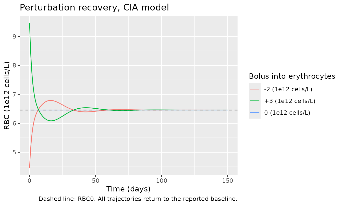
Replicate published figures
# rHuEPO doses in mIU/kg (1350 IU/kg = 1.35e6 mIU/kg).
epo_dose <- c("no treatment" = 0, "450 IU/kg" = 4.5e5, "1350 IU/kg" = 1.35e6)

# CKD: three times weekly for 2 weeks (Mon/Wed/Fri pattern), Methods.
ckd_dose_times <- c(0, 2, 4, 7, 9, 11) * 24

ckd_events <- function(amt, times) {
  ev <- rxode2::et(amt = 0, cmt = "central", time = 0)
  if (amt > 0) for (tt in ckd_dose_times) ev <- rxode2::et(ev, amt = amt, cmt = "central", time = tt)
  obs_at(ev, times)
}

# CIA: carboplatin 60 mg/kg = 6e4 ug/kg at t = 0, rHuEPO one week later.
t_epo <- 168
cia_events <- function(amt, times) {
  ev <- rxode2::et(amt = 6e4, cmt = "central_carb", time = 0)
  if (amt > 0) ev <- rxode2::et(ev, amt = amt, cmt = "central", time = t_epo)
  obs_at(ev, times)
}

sim_arms <- function(mod, evfun, times) {
  purrr_free <- lapply(names(epo_dose), function(nm) {
    s <- solve_det(mod, evfun(epo_dose[[nm]], times))
    s$arm <- nm
    s
  })
  out <- dplyr::bind_rows(purrr_free)
  out$arm <- factor(out$arm, levels = names(epo_dose))
  out
}
Figure 2A – ERFE over 24 h after the first rHuEPO dose, CKD rats
ckd_24 <- sim_arms(ckd, ckd_events, seq(0, 24, by = 0.25))

ggplot(ckd_24, aes(time, erfe, colour = arm)) +
  geom_line() +
  scale_x_continuous(breaks = c(0, 4, 8, 10, 12, 16, 20, 24)) +
  labs(x = "Time after treatment (h)", y = "ERFE (ng/mL)", colour = NULL,
       title = "Figure 2A -- ERFE kinetics in CKD rats",
       caption = paste("Replicates Figure 2A of Zhang 2025 (and the model curves of Figure 7A).",
                       "Observed: single circadian peak with saline; an additional early",
                       "peak near 4 h with rHuEPO."))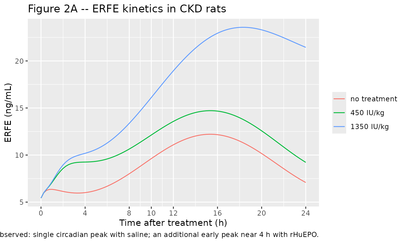
Figure 2D – ERFE over 24 h after rHuEPO, CIA rats
Time is re-referenced to the rHuEPO injection at 168 h so the axis matches the published panel.
cia_24 <- sim_arms(cia, cia_events, t_epo + seq(0, 24, by = 0.25))
cia_24$t_rel <- cia_24$time - t_epo

ggplot(cia_24, aes(t_rel, erfe, colour = arm)) +
  geom_line() +
  scale_x_continuous(breaks = c(0, 4, 8, 10, 12, 16, 20, 24)) +
  labs(x = "Time after rHuEPO (h)", y = "ERFE (ng/mL)", colour = NULL,
       title = "Figure 2D -- ERFE kinetics in CIA rats",
       caption = paste("Replicates Figure 2D of Zhang 2025 (and the model curves of Figure 7B).",
                       "The saline arm shows the characteristic early dip: circulating ERFE",
                       "starts at erfe_base(0) and relaxes toward the gain-scaled cosinor."))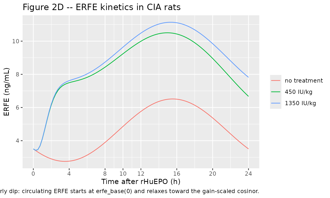
Figures 2B, 2C / 6B, 6C – long-term hemoglobin and RBC, CKD rats
ckd_long <- sim_arms(ckd, ckd_events, seq(0, 34 * 24, by = 4))

ckd_long |>
  dplyr::select(time, arm, HGB = hb, RBC = erythrocytes) |>
  tidyr::pivot_longer(c(HGB, RBC), names_to = "output", values_to = "value") |>
  ggplot(aes(time / 24, value, colour = arm)) +
  geom_line() +
  facet_wrap(~output, scales = "free_y") +
  labs(x = "Time after first rHuEPO dose (days)", y = NULL, colour = NULL,
       title = "Figures 2B, 2C -- hemoglobin (g/dL) and RBC (1e12 cells/L), CKD rats",
       caption = paste("Replicates Figures 2B/2C and the pcVPC medians of Figures 6B/6C.",
                       "The simulated response overshoots the published one; see Errata."))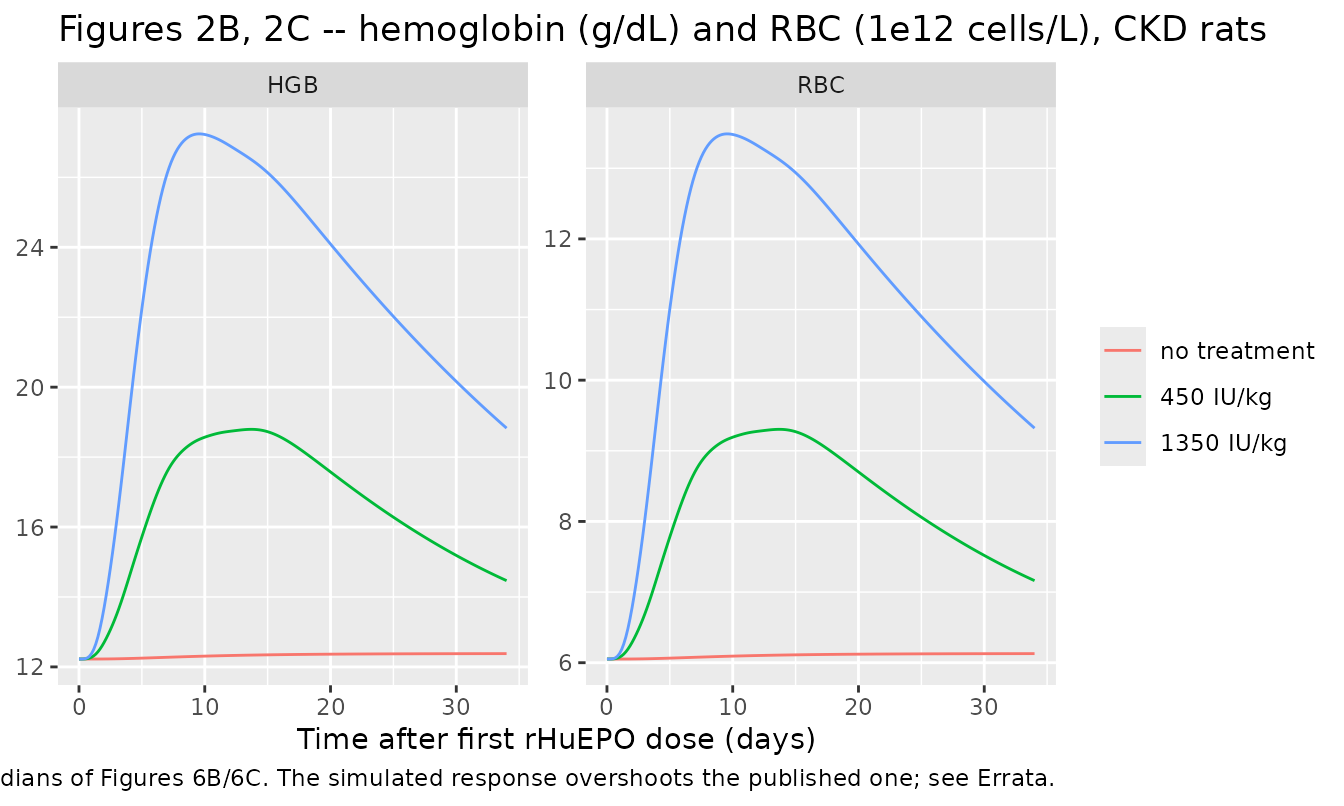
Figures 2E, 2F / 6E, 6F – long-term hemoglobin and RBC, CIA rats
cia_long <- sim_arms(cia, cia_events, seq(0, 32 * 24, by = 4))

cia_long |>
  dplyr::select(time, arm, HGB = hb, RBC = erythrocytes) |>
  tidyr::pivot_longer(c(HGB, RBC), names_to = "output", values_to = "value") |>
  ggplot(aes(time, value, colour = arm)) +
  geom_line() +
  geom_vline(xintercept = t_epo, linetype = "dotted") +
  facet_wrap(~output, scales = "free_y") +
  labs(x = "Time after carboplatin (h)", y = NULL, colour = NULL,
       title = "Figures 2E, 2F -- hemoglobin (g/dL) and RBC (1e12 cells/L), CIA rats",
       caption = paste("Replicates Figures 2E/2F and the pcVPC medians of Figures 6E/6F.",
                       "Dotted line: rHuEPO injection at 168 h. rHuEPO has no effect on",
                       "proliferation in the CIA model (Figure 1B), so the three arms",
                       "coincide on both hematological outputs -- exactly as the paper's",
                       "structure implies."))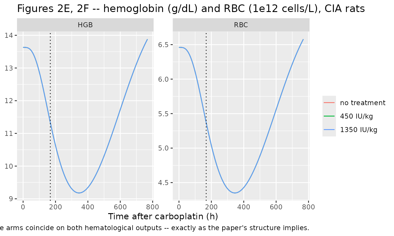
Figure S6 – simulated erythroblast (P3) time course, CIA rats
The paper’s mechanistic claim is that carboplatin drives the ERFE-producing erythroblast pool to a nadir by the time rHuEPO is given, blunting the ERFE response. Figure S6 is the direct test.
p3 <- solve_det(cia, cia_events(0, seq(0, 770, by = 4)))

ggplot(p3, aes(time, precursor3)) +
  geom_line() +
  geom_vline(xintercept = t_epo, linetype = "dotted", colour = "red") +
  labs(x = "Time after carboplatin (h)", y = "P3 (erythroblasts, 1e12 cells/L)",
       title = "Figure S6 -- simulated P3 time course, CIA rats",
       caption = "Replicates Figure S6 of Zhang 2025. Dotted red line: rHuEPO administration.")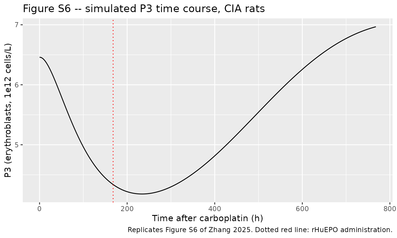
data.frame(
  quantity = c("P3 at t = 0", "P3 nadir", "nadir time (h)",
               "P3 at rHuEPO dose (168 h)", "P3 at 770 h"),
  simulated = signif(c(p3$precursor3[1], min(p3$precursor3),
                       p3$time[which.min(p3$precursor3)],
                       p3$precursor3[p3$time == t_epo],
                       p3$precursor3[nrow(p3)]), 4),
  published_figS6 = c("~6.95", "~4.2", "~230-260", "~4.25", "~6.95")
) |>
  dplyr::rename("Quantity" = quantity, "Simulated" = simulated,
                "Figure S6 (digitised)" = published_figS6) |>
knitr::kable(caption = "Simulated vs published P3 trajectory (published values read off Figure S6).")| Quantity | Simulated | Figure S6 (digitised) |
|---|---|---|
| P3 at t = 0 | 6.460 | ~6.95 |
| P3 nadir | 4.179 | ~4.2 |
| nadir time (h) | 232.000 | ~230-260 |
| P3 at rHuEPO dose (168 h) | 4.337 | ~4.25 |
| P3 at 770 h | 6.967 | ~6.95 |
Figure 7A – ERFE at three levels of rHuEPO responsiveness, CKD rats
Figure 7A varies EC50 over the three levels the paper
names – high (10), medium (100) and low (1360, the CKD estimate) – with
every other parameter at its estimate. The ordering and shape reproduce;
the amplitudes inherit the CKD erythroid over-prediction
documented in the Errata, because rHuEPO stimulation grows
precursor3 and ERFE production is proportional to it.
ec50_levels <- c("high responsiveness (EC50 = 10)" = 10,
                 "medium responsiveness (EC50 = 100)" = 100,
                 "low responsiveness (EC50 = 1360, CKD estimate)" = 1360)

fig7a <- lapply(names(epo_dose), function(arm) {
  lapply(names(ec50_levels), function(lev) {
    s <- rxode2::rxSolve(
      ckd, ckd_events(epo_dose[[arm]], seq(0, 24, by = 0.25)),
      params = c(lec50 = log(ec50_levels[[lev]])),
      useLinCmt = FALSE, returnType = "data.frame"
    )
    s$arm <- arm; s$responsiveness <- lev
    s
  }) |> dplyr::bind_rows()
}) |> dplyr::bind_rows()

fig7a$arm <- factor(fig7a$arm, levels = names(epo_dose))
fig7a$responsiveness <- factor(fig7a$responsiveness, levels = names(ec50_levels))

ggplot(fig7a, aes(time, erfe, colour = responsiveness)) +
  geom_line() +
  facet_wrap(~arm) +
  theme(legend.position = "bottom", legend.direction = "vertical") +
  labs(x = "Time (h)", y = "ERFE (ng/mL)", colour = NULL,
       title = "Figure 7A -- impaired rHuEPO responsiveness blunts ERFE, CKD rats",
       caption = "Replicates Figure 7A of Zhang 2025.")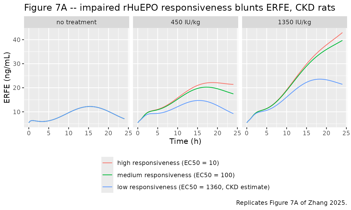
Figure 7B – ERFE at three levels of erythroblast mass, CIA rats
ERFE production enters Eq 19 as
ktr * precursor3 * emax * Cc / (ec50 + Cc), so multiplying
A(P3) by k – the paper’s stated manipulation – is
algebraically identical to multiplying Emax by k.
That is how the three precursor-mass levels are produced here. rHuEPO
does not act on proliferation in the CIA model, so this panel is free of
the CKD over-prediction.
mass_levels <- c("low precursor cell mass (x1)" = 1,
                 "medium precursor cell mass (x2)" = 2,
                 "high precursor cell mass (x3)" = 3)
emax_cia <- exp(cia$theta[["lemax"]])

fig7b <- lapply(names(epo_dose), function(arm) {
  lapply(names(mass_levels), function(lev) {
    s <- rxode2::rxSolve(
      cia, cia_events(epo_dose[[arm]], t_epo + seq(0, 24, by = 0.25)),
      params = c(lemax = log(emax_cia * mass_levels[[lev]])),
      useLinCmt = FALSE, returnType = "data.frame"
    )
    s$t_rel <- s$time - t_epo
    s$arm <- arm; s$mass <- lev
    s
  }) |> dplyr::bind_rows()
}) |> dplyr::bind_rows()

fig7b$arm <- factor(fig7b$arm, levels = names(epo_dose))
fig7b$mass <- factor(fig7b$mass, levels = names(mass_levels))

ggplot(fig7b, aes(t_rel, erfe, colour = mass)) +
  geom_line() +
  facet_wrap(~arm) +
  theme(legend.position = "bottom", legend.direction = "vertical") +
  labs(x = "Time (h)", y = "ERFE (ng/mL)", colour = NULL,
       title = "Figure 7B -- reduced precursor cell mass blunts ERFE, CIA rats",
       caption = "Replicates Figure 7B of Zhang 2025.")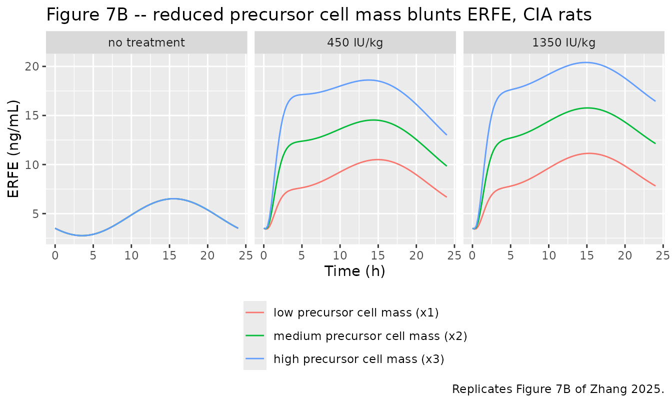
Comparison against published values
Zhang 2025 reports no NCA table, so PKNCA is not the right validation for either model (both are mechanistic turnover models with no drug-concentration observations at all). The comparison below is against values read off the published figures. Figure-digitised references carry roughly +/- 0.5 units of reading error, so a 20% tolerance is used.
ckd_1350 <- ckd_long[ckd_long$arm == "1350 IU/kg", ]
ckd_450  <- ckd_long[ckd_long$arm == "450 IU/kg", ]
ckd_none <- ckd_long[ckd_long$arm == "no treatment", ]
ckd24_1350 <- ckd_24[ckd_24$arm == "1350 IU/kg", ]
ckd24_450  <- ckd_24[ckd_24$arm == "450 IU/kg", ]
ckd24_none <- ckd_24[ckd_24$arm == "no treatment", ]
cia24_1350 <- cia_24[cia_24$arm == "1350 IU/kg", ]
cia24_none <- cia_24[cia_24$arm == "no treatment", ]
cia_none   <- cia_long[cia_long$arm == "no treatment", ]

at <- function(d, tt, col) d[[col]][which.min(abs(d$time - tt))]

# Drug-induced ERFE at 4 h, corrected for the circadian baseline by
# subtracting the saline arm at the same clock time. This is the quantity the
# paper's biomarker analysis uses ("the change of ERFE at 4 h post-rHuEPO"),
# and it removes the reading error in the circadian phase of the raw figures.
induction4 <- function(arm_df, saline_df, t0 = 0) {
  at(arm_df, t0 + 4, "erfe") - at(saline_df, t0 + 4, "erfe")
}

cmp <- tibble::tribble(
  ~metric,                                             ~simulated,                                   ~published, ~source,
  "CKD ERFE baseline at t = 0 (ng/mL)",                at(ckd24_none, 0, "erfe"),                    5.4,        "Fig 7A panel 0",
  "CKD ERFE circadian peak, saline (ng/mL)",           max(ckd24_none$erfe),                         12.2,       "Fig 7A panel 0",
  "CKD ERFE circadian peak time, saline (h)",          ckd24_none$time[which.max(ckd24_none$erfe)],  15.0,       "Fig 7A panel 0",
  "CKD ERFE at 24 h, saline (ng/mL)",                  at(ckd24_none, 24, "erfe"),                   7.0,        "Fig 7A panel 0",
  "CKD ERFE induction at 4 h, 450 IU/kg (ng/mL)",      induction4(ckd24_450, ckd24_none),            2.5,        "Fig 2A",
  "CKD ERFE induction at 4 h, 1350 IU/kg (ng/mL)",     induction4(ckd24_1350, ckd24_none),           4.5,        "Fig 2A",
  "CKD HGB baseline (g/dL)",                           at(ckd_none, 0, "hb"),                        12.4,       "Fig 2B",
  "CKD HGB peak, 450 IU/kg (g/dL)",                    max(ckd_450$hb),                              16.0,       "Fig 2B",
  "CKD HGB peak, 1350 IU/kg (g/dL)",                   max(ckd_1350$hb),                             20.0,       "Fig 2B / 6B",
  "CKD RBC peak, 1350 IU/kg (1e12 cells/L)",           max(ckd_1350$erythrocytes),                   9.5,        "Fig 2C / 6C",
  "CIA ERFE baseline at rHuEPO dose (ng/mL)",          at(cia24_none, t_epo, "erfe"),                3.4,        "Fig 7B panel 0",
  "CIA ERFE circadian peak, saline (ng/mL)",           max(cia24_none$erfe),                         6.5,        "Fig 7B panel 0",
  "CIA ERFE induction at 4 h, 1350 IU/kg (ng/mL)",     induction4(cia24_1350, cia24_none, t_epo),    5.0,        "Fig 2D",
  "CIA HGB baseline (g/dL)",                           at(cia_none, 0, "hb"),                        13.0,       "Fig 6E",
  "CIA HGB nadir (g/dL)",                              min(cia_none$hb),                             8.8,        "Fig 6E",
  "CIA HGB nadir time (h)",                            cia_none$time[which.min(cia_none$hb)],        350,        "Fig 6E",
  "CIA RBC nadir (1e12 cells/L)",                      min(cia_none$erythrocytes),                   3.9,        "Fig 6F"
)

cmp <- cmp |>
  dplyr::mutate(
    simulated = signif(simulated, 4),
    diff_pct = signif(100 * (simulated / published - 1), 3),
    flag = ifelse(abs(diff_pct) > 20, "*", "")
  )

cmp |>
  dplyr::rename(
    "Metric" = metric, "Simulated" = simulated,
    "Published (digitised)" = published, "Source" = source,
    "Difference (%)" = diff_pct, "Over 20%" = flag
  ) |>
  knitr::kable(align = c("l", "r", "r", "l", "r", "l"),
caption = "Simulated vs published. * differs from the digitised reference by more than 20%.")| Metric | Simulated | Published (digitised) | Source | Difference (%) | Over 20% |
|---|---|---|---|---|---|
| CKD ERFE baseline at t = 0 (ng/mL) | 5.429 | 5.4 | Fig 7A panel 0 | 0.537 | |
| CKD ERFE circadian peak, saline (ng/mL) | 12.210 | 12.2 | Fig 7A panel 0 | 0.082 | |
| CKD ERFE circadian peak time, saline (h) | 15.250 | 15.0 | Fig 7A panel 0 | 1.670 | |
| CKD ERFE at 24 h, saline (ng/mL) | 7.084 | 7.0 | Fig 7A panel 0 | 1.200 | |
| CKD ERFE induction at 4 h, 450 IU/kg (ng/mL) | 3.248 | 2.5 | Fig 2A | 29.900 | * |
| CKD ERFE induction at 4 h, 1350 IU/kg (ng/mL) | 4.177 | 4.5 | Fig 2A | -7.180 | |
| CKD HGB baseline (g/dL) | 12.230 | 12.4 | Fig 2B | -1.370 | |
| CKD HGB peak, 450 IU/kg (g/dL) | 18.790 | 16.0 | Fig 2B | 17.400 | |
| CKD HGB peak, 1350 IU/kg (g/dL) | 27.240 | 20.0 | Fig 2B / 6B | 36.200 | * |
| CKD RBC peak, 1350 IU/kg (1e12 cells/L) | 13.490 | 9.5 | Fig 2C / 6C | 42.000 | * |
| CIA ERFE baseline at rHuEPO dose (ng/mL) | 3.505 | 3.4 | Fig 7B panel 0 | 3.090 | |
| CIA ERFE circadian peak, saline (ng/mL) | 6.516 | 6.5 | Fig 7B panel 0 | 0.246 | |
| CIA ERFE induction at 4 h, 1350 IU/kg (ng/mL) | 4.851 | 5.0 | Fig 2D | -2.980 | |
| CIA HGB baseline (g/dL) | 13.630 | 13.0 | Fig 6E | 4.850 | |
| CIA HGB nadir (g/dL) | 9.178 | 8.8 | Fig 6E | 4.300 | |
| CIA HGB nadir time (h) | 344.000 | 350.0 | Fig 6E | -1.710 | |
| CIA RBC nadir (1e12 cells/L) | 4.350 | 3.9 | Fig 6F | 11.500 |
starred <- cmp$metric[cmp$flag == "*"]
starred
#> [1] "CKD ERFE induction at 4 h, 450 IU/kg (ng/mL)"
#> [2] "CKD HGB peak, 1350 IU/kg (g/dL)"
#> [3] "CKD RBC peak, 1350 IU/kg (1e12 cells/L)"
# Only the CKD long-term erythroid amplitude and the 450 IU/kg CKD ERFE
# induction may exceed the 20% band; everything else must agree.
stopifnot(all(grepl("^CKD (HGB peak|RBC peak|ERFE induction at 4 h, 450)", starred)))
The circadian ERFE arm of both models reproduces the published curves closely: baseline, circadian amplitude, acrophase and the 24-h value agree to within a few percent in both diseases, and the drug-induced 4-h ERFE increment – the quantity the paper’s biomarker analysis is built on – agrees within about 7% at 1350 IU/kg in both models. The CIA erythroid arm reproduces the hemoglobin and RBC nadir magnitude and timing and the Figure S6 erythroblast trajectory. The starred rows are the CKD long-term erythroid amplitude (and, at the lower CKD dose, the ERFE increment that follows from it), discussed next. Nothing was tuned to close them.
At 450 IU/kg the CIA model predicts nearly the same 4-h ERFE
induction as at 1350 IU/kg, whereas the observed means of Figure 2D show
a 4-h peak only in the high-dose group. With
EC50 = 126 mIU/mL and Cc(0+) of 7.4e3-2.2e4
mIU/mL the induction is saturated at both doses, so the model cannot
separate them – and the authors’ own Figure 7B shows the same
near-coincidence of the two dose panels. This is a property of the
published EC50, not of the encoding.
Assumptions and deviations
The CKD erythroid response over-predicts the published one
Simulating the CKD model with KEPO = 0.0106 as printed
in Table 1 gives a hemoglobin peak of about 27 g/dL after 1350 IU/kg
three times weekly, against about 20 g/dL in both the observed data
(Figure 2B) and the authors’ own pcVPC (Figure 6B). RBC over-predicts in
proportion. The discrepancy is confined to this one term:
- The circadian ERFE sub-model reproduces the saline panels of Figures 7A and 7B essentially exactly (baseline, amplitude, acrophase, 24-h value, and the characteristic early dip in CIA).
- The drug-induced 4-h ERFE increment – the paper’s biomarker readout – agrees within about 7% at 1350 IU/kg in both models.
- The CIA erythroid model, which uses
Kcarbrather thanKEPO, reproduces the hemoglobin and RBC nadir magnitudes and timing and the Figure S6 P3 trajectory (nadir 4.18 vs about 4.2 at 232 h vs about 230-260 h). - Only the CKD
(1 + KEPO * Cc)stimulation of progenitor production is affected. Because ERFE production is proportional toprecursor3, the CKD Figure 7A amplitudes at 15-24 h inherit the same factor (roughly 1.7x the published peaks) even though the ordering by responsiveness is correct; the early (4 h) ERFE values, which the biomarker analysis uses, are beforeprecursor3has had time to grow and are therefore unaffected.
Diagnostics: reproducing Figures 6B/6C requires the stimulation term
to be about 0.3-0.4 times smaller than the printed equation and Table S1
units give. A rat of 0.25-0.30 kg is exactly that factor, which is
consistent with the upstream model having evaluated
A1 / VEPO with A1 as an
absolute amount (mIU) while VEPO is
reported per kg (mL/kg, Table S1) – i.e. a per-kg /
absolute mismatch in the concentration that drives progenitor
stimulation. This is a hypothesis, not a documented fact, and the paper
states the per-kg units explicitly, so the packaged model
encodes the printed equation and the printed Table S1 units
without a weight correction. Nothing was tuned. Users
reproducing Figure 6B/6C should be aware that the long-term CKD
hemoglobin and RBC amplitude is high by roughly a factor of two in the
increment over baseline; the ERFE predictions – the subject of the paper
– are unaffected at the early time points that the biomarker analysis
uses.
Values and readings not stated by the paper
-
TRET(reticulocyte lifespan) appears inkIN0 = RBC0 / ((TRBC + TRET) * AMPN * AMPC)(Methods, after Eq 11) but is reported nowhere in the paper or its Supporting Information. It is taken equal to the precursor lifespanT, becauseprecursor4is the reticulocyte pool in this model and its residence time isT. That choice makeskIN0exactlyprecursor1(0) / T, closing the progenitor balance at the paper’s own printed initial conditions. The residual consequence is quantified above: a 1.3% upward drift in baseline hemoglobin over 34 days, because the printed initial conditionerythrocytes(0) = RBC0 - RBC0*T/(TRBC+T)makes the feedback term(RBC0/erythrocytes)^gammaequal 1.065 rather than 1 at time zero. SettingTRET = 104.6 hinstead would remove the drift exactly; that value is a back-solve, not a published number, and is not used. -
RET0is the printed initial condition forprecursor3(Methods, after Eq 11) and is likewise never reported. The zero-net-flux steady state of Eq 8 fixes it atRBC0 * T / (TRBC + T), which is what the model uses. -
kout,ERFEappears in the definition ofkCINEas a symbol distinct fromkout, but only oneKoutis tabulated. Settingkout,ERFE = koutis what makes the cosinor an exact solution of Eq 18; the mass-balance check above confirms it numerically. -
Residual-error scale. Tables 1 and 2 report
sigmafor RBC / HGB / ERFE in a column headed “sigma (%)” with values 0.495 / 1.03 / 1.54 (CKD) and 0.748 / 1.51 / 2.2 (CIA). Read as CV percentages directly, the resulting prediction bands are roughly 20-fold narrower than the pcVPC bands of Figure 6; read as unitless variances they give CV 70-148%, far wider. The reading used here is that the tabulated number is the proportional-error variance expressed as a percentage, soCV = sqrt(value / 100), giving 7.0 / 10.1 / 12.4% (CKD) and 8.6 / 12.3 / 14.8% (CIA). Those match the width of all six published pcVPC panels. This is an interpretation of an ambiguous table, not a stated fact. -
Kcarbunits. Table 2 printsh-1, but1 - Kcarb * (A1CAR / Vcarb)requiresKcarbto be reciprocal-concentration. With carboplatin concentration in ug/mL (= mg/L, the conventional unit) the printed value 0.172 mL/ug reproduces the observed hemoglobin nadir; in mg/mL it would produce essentially no myelosuppression. The dimensional-analysis table above records the reading. -
Emaxunits. Tables 1 and 2 printcell-1; the termktr * precursor3 * emaxmust have units ng/mL/h, soEmaxis(ng/mL) / (1e12 cells/L). -
Hemoglobin equation. Eqs 11 and 17 are typeset as
dAHGB/dt = MCH * ARBC / 10, which is dimensionally a rate and would grow without bound. Figure 1 draws HGB as derived from RBC, andMCH * RBC0 / 10reproduces the observed baselines (12.4 and 13.6 g/dL), so the relation is encoded algebraically. -
Circadian phase reference.
tpeakis applied to the model time origin, i.e. the time of the rHuEPO or saline injection, matching the paper’s “Time after treatment” axis. The injection clock time is not reported. - CKD dosing schedule. “Three times weekly for 2 weeks” is implemented as days 0, 2, 4, 7, 9, 11 (a Monday/Wednesday/Friday pattern). The exact calendar is not tabulated.
-
Figure 7 reproduction. Figure 7A varies
EC50over the three levels the Methods name (10, 100, 1360) with the coupled model, as the paper did. Figure 7B multipliesA(P3)by 1, 2 and 3; because ERFE production enters Eq 19 asktr * precursor3 * emax * ..., that is reproduced by scalingEmaxinstead, which is algebraically identical and does not perturb the erythroid chain. - Published reference values are figure-digitised. Zhang 2025 tabulates parameter estimates but no summary statistics of the observed profiles, so every “published” number in the comparison table was read off Figures 2, 6, 7 or S6 with roughly +/- 0.5 units of reading error.
Naming
Three erythroferrone states (erfe,
erfe_base, erfe_induced) and the three
carboplatin disposition states (central_carb,
peripheral1_carb, peripheral2_carb) are
declared through paper_specific_compartments rather than
registered as new canonical names. Two register additions are proposed
for the maintainer’s consideration and deliberately not
made here:
-
erfeas a canonical circulating-erythroferrone PD-output compartment, alongside the existinghep(hepcidin) andironentries – ERFE is the direct upstream suppressor of hepcidin, so the three belong together. -
carbas a canonical carboplatin sibling-drug suffix, alongsidefebx,lesn,roc,pyra,mer,sbtanddex. Carboplatin is co-administered with rHuEPO and is not a metabolite of it. Note thatcarbalready occurs as a compartment token for carbohydrate pools inGuiastrennec_2016_gastric_emptying.R; the register permits the same token under two different Types (see themerentry).
Everything else uses existing canonical names: central /
peripheral1 (rHuEPO), precursor1 …
precursor4, erythrocytes,
transit1 / transit2, hb, and the
parameter canonicals lvmax / lkm /
lvc / lkel / lk12 /
lk21 / lmtt / ltp /
lgamma / lrbase_rbc / lslope /
lkin-family lkout / lktr /
lemax / lec50 and the circadian trio
lrm / lra / ltacro.