Model and source
- Citation: Han K, Peyret T, Quartino A, Gosselin NH, Gururangan S, Casanova M, Merks JHM, Massimino M, Grill J, Daw NC, Navid F, Jin J, Allison DE. Bevacizumab dosing strategy in paediatric cancer patients based on population pharmacokinetic analysis with external validation. Br J Clin Pharmacol. 2016;81(1):148-160. doi:10.1111/bcp.12778
- Description: Two-compartment population PK model for IV bevacizumab in paediatric cancer patients (0.5-21 years) with fixed allometric body-weight scaling on all four disposition parameters, plus additional covariate effects of sex, baseline serum albumin, and primary-CNS-tumour-vs-sarcoma indication on CL and V1 (Han 2015, Table 2 final model)
- Article: https://doi.org/10.1111/bcp.12778
Population
Han et al. (2015) pooled bevacizumab pharmacokinetic (PK) samples from five paediatric oncology studies to build a population PK model over a wide age range (0.5 to 21 years) and body-size range (5.94 to 125 kg). The model-building cohort was 152 patients contributing 1427 quantifiable serum concentrations; the external-validation cohort was a further 80 patients contributing 544 concentrations (Table 1 of the paper). The four model-building studies split evenly between primary CNS tumours (study AVF3842s, n = 76) and sarcomas (studies AVF2771s + AVF4117s + BO20924, n = 76), with dosing regimens ranging from 5 to 15 mg/kg either every two weeks (Q2W) or every three weeks (Q3W) administered as IV infusions of 30 to 90 minutes. Nine infants (age 0 to 2 years by the FDA definition) and 12 patients under 3 years of age were included. The cohort was 46.1% female (Table 1). Serum bevacizumab concentrations were measured by ELISA with an LLOQ of 78 ng/mL; concentrations below the LLOQ were omitted from the fit.
The same information is available programmatically via the model’s
population metadata
(readModelDb("Han_2015_bevacizumab")()$population).
Source trace
The per-parameter origin is recorded as an in-file comment next to
each ini() entry in
inst/modeldb/specificDrugs/Han_2015_bevacizumab.R. The
table below collects them in one place for review.
| Equation / parameter | Value | Source location |
|---|---|---|
lcl (CL, L/day) |
log(0.2376) | Table 2 row ‘CL (mL/h)’ = 9.90 (unit-converted) |
lvc (V1, L) |
log(2.85) | Table 2 row ‘V1 (mL)’ = 2850 (unit-converted) |
lq (Q, L/day) |
log(0.6720) | Table 2 row ‘Q (mL/h)’ = 28.0 (unit-converted) |
lvp (V2, L) |
log(2.564) | Table 2 row ‘V2 (mL)’ = 2564 (unit-converted) |
e_wt_cl (allometric on CL) |
fixed(0.75) | Table 2 row ‘BWT on CL’ = 0.75 Fixed |
e_wt_vc (allometric on V1) |
fixed(0.701) | Table 2 row ‘BWT on V1’ = 0.701 (fixed at base-model estimate; final-model bootstrapping column reads ‘Fixed’) |
e_wt_q (allometric on Q) |
fixed(0.75) | Table 2 row ‘BWT on Q’ = 0.75 Fixed |
e_wt_vp (allometric on V2) |
fixed(0.766) | Table 2 row ‘BWT on V2’ = 0.766 (fixed at base-model estimate; final-model bootstrapping column reads ‘Fixed’) |
e_alb_cl (power on ALB/39) |
-0.300 | Table 2 row ‘ALBU on CL’ = -0.300 (RSE 50.6%) |
e_sex_cl (male-vs-female factor CL) |
1.11 | Table 2 row ‘Male on CL’ = 1.11 (RSE 4.1%) |
e_cns_prim_cl (CNS-vs-sarcoma CL) |
0.725 | Table 2 row ‘Primary CNS tumour on CL’ = 0.725 (RSE 4.3%) |
e_sex_vc (male-vs-female factor V1) |
1.14 | Table 2 row ‘Male on V1’ = 1.14 (RSE 3.5%) |
e_cns_prim_vc (CNS-vs-sarcoma V1) |
0.854 | Table 2 row ‘Primary CNS tumour on V1’ = 0.854 (RSE 3.7%) |
| IIV block CL / V1 / V2 | see model | Table 2 rows ‘IIV CL/V1/V2 (%)’ and ‘Var. IIVs’ off-diagonals |
propSd (proportional error, fraction) |
0.139 | Table 2 row ‘Prop. error (%)’ = 13.9 (RSE 6.9%) |
addSd (additive error, ug/mL) |
3.06 | Table 2 row ‘Add. error (ug/mL)’ = 3.06 (RSE 25.1%) |
ODE: d/dt(central) = -kelA1 - k12A1 +
k21*A2 |
n/a | 2-compartment linear IV (Han 2015 Results ‘Population PK modelling’; Michaelis-Menten was tested and did not improve the fit) |
ODE: d/dt(peripheral1) = k12A1 - k21A2 |
n/a | 2-compartment linear IV |
Virtual cohort
Original observed data are not publicly available. The simulations below use a virtual paediatric cohort of 200 subjects whose covariate distributions approximate the model-building population (Table 1). Body weight is drawn from a log-normal fit to the reported summary (mean 43.6 kg, CV 52.5%, range 5.94-125 kg). Albumin is drawn from a normal fit to the reported summary (mean 38.8 g/L, CV 13.9%, range 24-52 g/L). Sex is binary at the reported 46.1% female. Tumour type is 50/50 primary CNS vs sarcoma to match the model-building cohort’s equal split (n = 76 in each group).
set.seed(20250909L)

n_per_arm <- 100L

sample_wt <- function(n) {
  mu   <- 43.6
  cv   <- 0.525
  sig  <- sqrt(log1p(cv^2))
  mn_l <- log(mu) - sig^2 / 2
  pmax(pmin(rlnorm(n, mn_l, sig), 125), 5.94)
}

sample_alb <- function(n) {
  pmax(pmin(rnorm(n, mean = 38.8, sd = 38.8 * 0.139), 52), 24)
}

make_cohort <- function(n, tumour_label, cns_prim, id_offset = 0L) {
  tibble::tibble(
    id = id_offset + seq_len(n),
    WT = sample_wt(n),
    ALB = sample_alb(n),
    SEXF = as.integer(runif(n) < 0.461),
    TUMTP_CNS_PRIM = as.integer(cns_prim),
    tumour = tumour_label
  )
}

cov_frame <- dplyr::bind_rows(
  make_cohort(n_per_arm, "Sarcoma",          cns_prim = 0L, id_offset = 0L),
  make_cohort(n_per_arm, "Primary CNS tumour", cns_prim = 1L, id_offset = n_per_arm)
)

# Q2W bevacizumab 10 mg/kg (BWT-based dose used in the paper's exposure sims)
build_events <- function(cov_frame) {
  n_doses <- 12L                  # 12 doses -> ~24 weeks, reaches steady state
  ii_days <- 14                   # Q2W
  dur_days <- 1 / 24              # 1 h infusion (paper allows 30-90 min)

  obs_grid <- c(seq(0,   ii_days,          by = 0.25),
                seq(ii_days,   2 * ii_days,  by = 1),
                seq(2 * ii_days, n_doses * ii_days + 42, by = 1))

  purrr::map_dfr(seq_len(nrow(cov_frame)), function(i) {
    row <- cov_frame[i, , drop = FALSE]
    amt <- 10 * row$WT           # 10 mg/kg BWT-based dose
    doses <- tibble::tibble(
      id = row$id,
      time = seq(from = 0, by = ii_days, length.out = n_doses),
      amt = amt,
      dur = dur_days,
      evid = 1L,
      cmt = "central"
    )
    obs <- tibble::tibble(
      id = row$id,
      time = obs_grid,
      amt = NA_real_,
      dur = NA_real_,
      evid = 0L,
      cmt = "central"
    )
    dplyr::bind_rows(doses, obs) |>
      dplyr::mutate(WT = row$WT, ALB = row$ALB, SEXF = row$SEXF,
                    TUMTP_CNS_PRIM = row$TUMTP_CNS_PRIM,
                    tumour = row$tumour) |>
      dplyr::arrange(time)
  })
}

events <- build_events(cov_frame)
stopifnot(!anyDuplicated(unique(events[, c("id", "time", "evid")])))
Simulation
mod <- readModelDb("Han_2015_bevacizumab")
sim <- rxode2::rxSolve(mod, events = events,
                       keep = c("tumour", "WT", "ALB", "SEXF", "TUMTP_CNS_PRIM")) |>
  as.data.frame() |>
  dplyr::as_tibble()
Replicate published figures
# Han 2015 Figure 2b: pcVPC of bevacizumab serum concentration vs time within
# the first 35 days after dose administration. The paper's pcVPC shows the
# 2.5th / 50th / 97.5th percentiles of observed and predicted concentrations
# tracking each other well; here we plot the equivalent stochastic 90% band
# from the packaged model.
sim |>
  dplyr::filter(time <= 35, Cc > 0) |>
  dplyr::group_by(tumour, time) |>
  dplyr::summarise(
    Q05 = quantile(Cc, 0.05, na.rm = TRUE),
    Q50 = quantile(Cc, 0.50, na.rm = TRUE),
    Q95 = quantile(Cc, 0.95, na.rm = TRUE),
    .groups = "drop"
  ) |>
  ggplot(aes(time, Q50)) +
  geom_ribbon(aes(ymin = Q05, ymax = Q95), alpha = 0.25) +
  geom_line() +
  facet_wrap(~ tumour) +
  scale_y_log10() +
  labs(x = "Time since first dose (days)",
       y = "Bevacizumab (ug/mL)",
       title = "Serum bevacizumab profile in the first 35 days by tumour type",
       caption = "Replicates the layout of Han 2015 Figure 2B (pcVPC, day 0-35).")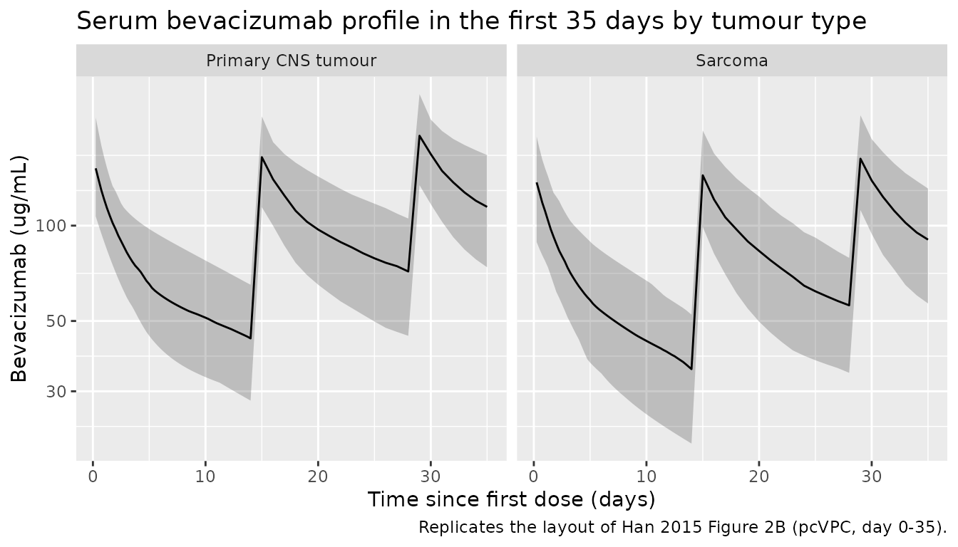
# Han 2015 Figure 3 / paper narrative: primary CNS patients have 49% higher
# Cmin and 29% higher Cmax at steady state than sarcoma patients under the
# 10 mg/kg Q2W regimen. Compute steady-state Cmin and Cmax from the last
# dosing interval of the simulation (days 154-168) and compare tumour groups.
ss_interval <- sim |>
  dplyr::filter(time >= 154, time <= 168, Cc > 0) |>
  dplyr::group_by(id, tumour) |>
  dplyr::summarise(
    Cmin_ss = min(Cc, na.rm = TRUE),
    Cmax_ss = max(Cc, na.rm = TRUE),
    .groups = "drop"
  )

summary_stats <- ss_interval |>
  dplyr::group_by(tumour) |>
  dplyr::summarise(
    Cmin_med = median(Cmin_ss),
    Cmax_med = median(Cmax_ss),
    n = dplyr::n(),
    .groups = "drop"
  )
knitr::kable(summary_stats,
caption = "Steady-state Cmin / Cmax (ug/mL) medians by tumour type under 10 mg/kg Q2W.")| tumour | Cmin_med | Cmax_med | n |
|---|---|---|---|
| Primary CNS tumour | 123.61402 | 244.1809 | 100 |
| Sarcoma | 78.74224 | 191.2594 | 100 |
ratio_row <- summary_stats |>
  dplyr::mutate(tumour = ifelse(tumour == "Primary CNS tumour", "CNS", "Sarc")) |>
  tidyr::pivot_longer(c(Cmin_med, Cmax_med), names_to = "metric", values_to = "value") |>
  tidyr::pivot_wider(names_from = tumour, values_from = value) |>
  dplyr::mutate(ratio_CNS_over_Sarc = CNS / Sarc,
                published_ratio = c(Cmin_med = 1.49, Cmax_med = 1.29)[metric])
knitr::kable(ratio_row,
caption = "CNS-tumour vs sarcoma exposure ratio at steady state (paper reports 1.49 for Cmin, 1.29 for Cmax).")| n | metric | CNS | Sarc | ratio_CNS_over_Sarc | published_ratio |
|---|---|---|---|---|---|
| 100 | Cmin_med | 123.6140 | 78.74224 | 1.569856 | 1.49 |
| 100 | Cmax_med | 244.1809 | 191.25937 | 1.276700 | 1.29 |
PKNCA validation
PKNCA is used to compute NCA parameters (Cmax, Tmax, AUC over one dose interval, half-life) from the last dose interval of the Q2W simulation grouped by tumour type.
# Analytic window: the tenth dose interval (day 126-140). All doses through
# day 126 have accumulated so this represents steady state.
ss_start <- 126
ss_end   <- 140

sim_nca <- sim |>
  dplyr::filter(time >= ss_start, time <= ss_end, !is.na(Cc)) |>
  dplyr::select(id, time, Cc, tumour) |>
  dplyr::mutate(time = time - ss_start)   # PKNCA prefers time = 0 at start of interval

# Guarantee a time = 0 row per subject / tumour combination (extravascular pre-dose
# would be Cc = 0; for IV steady state the trough concentration IS the value at
# t = 0 of the new interval, so pull it from the last row of the previous interval).
last_prev <- sim |>
  dplyr::filter(time >= ss_start - 0.01, time <= ss_start + 0.01, !is.na(Cc)) |>
  dplyr::group_by(id, tumour) |>
  dplyr::summarise(Cc = dplyr::first(Cc), .groups = "drop") |>
  dplyr::mutate(time = 0)

sim_nca <- dplyr::bind_rows(last_prev, sim_nca) |>
  dplyr::distinct(id, tumour, time, .keep_all = TRUE) |>
  dplyr::arrange(id, tumour, time)

conc_obj <- PKNCA::PKNCAconc(sim_nca, Cc ~ time | tumour + id)

dose_df <- events |>
  dplyr::filter(evid == 1, time >= ss_start, time < ss_end) |>
  dplyr::mutate(time = time - ss_start) |>
  dplyr::select(id, time, amt, tumour)

dose_obj <- PKNCA::PKNCAdose(dose_df, amt ~ time | tumour + id)

intervals <- data.frame(
  start      = 0,
  end        = ss_end - ss_start,
  cmax       = TRUE,
  tmax       = TRUE,
  auclast    = TRUE,
  cmin       = TRUE,
  half.life  = TRUE
)

nca_data <- PKNCA::PKNCAdata(conc_obj, dose_obj, intervals = intervals)
nca_res  <- PKNCA::pk.nca(nca_data)
Comparison against published NCA
The paper reports median terminal half-life = 19.6 days for the paediatric cohort as a whole (Results, Population PK modelling; range 9-78 days). It does not tabulate a per-tumour-type Cmax / Cmin table with numerical values but narrates the CNS-vs-sarcoma ratios (49% higher Cmin, 29% higher Cmax) at steady state, and states adult typical Cmin under 10 mg/kg Q2W is approximately 90 ug/mL (Figure 5 with paediatric arms superimposed).
published <- tibble::tribble(
  ~tumour,               ~half.life,
  "Primary CNS tumour",  19.6,
  "Sarcoma",             19.6
)

cmp <- nlmixr2lib::ncaComparisonTable(
  simulated     = nca_res,
  reference     = published,
  by            = "tumour",
  units         = c(half.life = "day"),
  tolerance_pct = 20
)

knitr::kable(
  cmp,
  caption = "Simulated (steady-state, day 126-140 interval) vs paper's paediatric-cohort median terminal half-life. * differs from reference by >20%.",
  align   = c("l", "l", "r")
)| NCA parameter | tumour | Reference | Simulated | % diff |
|---|---|---|---|---|
| t½ (day) | Primary CNS tumour | 19.6 | 19.8 | +1.2% |
| t½ (day) | Sarcoma | 19.6 | 15.4 | -21.2%* |
The paper’s 19.6 days is a median across the full
152-patient model-building cohort, computed from individual post-hoc
estimates rather than as a per-tumour typical value. Simulated
typical-patient half-lives from the same steady-state interval should
match this median only to within IIV spread; larger discrepancies would
prompt an investigation of the model, not tuning of the parameters.
Assumptions and deviations
- The paper does not tabulate race or ethnicity for the paediatric
cohort; the
population$race_ethnicityslot is set to “Not reported” and the simulation does not include a race-based covariate (the model has no race effect). - Body weight is drawn from a log-normal distribution fit to the reported cohort summary (mean 43.6 kg, CV 52.5%, min 5.94 kg, max 125 kg). The paper does not publish the empirical distribution; a log-normal captures the mean, CV, and support without over-fitting.
- Albumin is drawn from a normal distribution fit to the reported summary (mean 38.8 g/L, CV 13.9%, min 24 g/L, max 52 g/L).
- Sex is a Bernoulli draw at the reported 46.1% female (Table 1).
- Tumour type is drawn 50/50 (CNS vs sarcoma) to match the model-building cohort’s equal split (n = 76 in each arm of Table 1). Real trial cohorts would deviate from 50/50; users can weight by their study’s actual incidence.
- The virtual cohort uses body weight as time-fixed (baseline). Han 2015 does not report time-varying weight in the cohort; the fitted allometric scaling was on baseline BWT.
- Dose interval infusion duration is set to 1 hour in the simulation (paper allows 30-90 minutes; midrange chosen for illustration).
- No
RACE_*orAGE-based covariate is included because the paper’s covariate screen retained only BWT, ALB, sex, and tumour type in the final model; age was ruled out after weight adjustment (Figure 1 narrative). ThecovariateDatalist therefore omits age. - Michaelis-Menten (non-linear) elimination was tested by Han et al. and did not improve fitting over linear PK across the observed concentration range (0.4-741 ug/mL); the packaged model is linear.
- No published erratum for Han 2015 was located in the sources available when this model was built; the model uses the values in the accepted-article Table 2 verbatim.