Model and source
- Citation: Ji XW, Ji SM, He XR, Zhu X, Chen R, Lu W. Influences of renal function descriptors on population pharmacokinetic modeling of vancomycin in Chinese adult patients. Acta Pharmacol Sin. 2018;39(2):286-293. doi:10.1038/aps.2017.57 (published online 24 Aug 2017)
- Description: One-compartment IV (intermittent-infusion) population PK model for vancomycin in Chinese adult patients (Ji 2017). Clearance is scaled by raw Cockcroft-Gault creatinine clearance (centered linear term, reference 80 mL/min) and by age (power of (75/age), reference 75 years); the volume of distribution is a single typical value. Developed from steady-state trough therapeutic-drug-monitoring data.
- Article: Acta Pharmacol Sin 2018;39(2):286-293
The article was published online on 24 Aug 2017 (DOI
aps.2017.57) and appeared in the 2018 print volume; the
model file uses the online/DOI year (2017) in its name while the
reference field carries the full 2018 print citation.
Population
The model was developed from routine therapeutic-drug-monitoring data
on 160 hospitalized Chinese adults treated with intravenous vancomycin
(1000 mg every 12 h) at Beijing Hospital, Beijing, China (Ji 2017 Table
1); a further 58 patients were held out for external validation (218
patients in total). None were on renal replacement therapy. Median age
was 78 years (range 42-95), median body weight 65 kg (range 38-90), and
median Cockcroft-Gault creatinine clearance 58.02 mL/min (range
5.45-224.0). 54 of 160 model-building subjects (33.75%) were female. The
dataset contained 251 trough (Cmin) serum vancomycin concentrations
sampled before the next dose; each patient contributed at least one
sample (median 2, range 1-17). Concentrations were measured by TDx-FLx
fluorescence polarization immunoassay (LOQ 2.0 mg/L) and parameters
estimated in NONMEM 7 with FOCEI. The same information is available
programmatically via
readModelDb("Ji_2017_vancomycin")$population.
Source trace
Every numeric value in ini() carries an in-file comment
pointing to the Ji 2017 source location. The table below collects them
in one place for review.
| Equation / parameter | Value | Source location |
|---|---|---|
lcl (CL) |
2.829 L/h | Eq 16 / Table 3, row “CL (L/h)” (final model) |
lvc (V) |
52.14 L | Eq 17 / Table 3, row “V (L)” (final model) |
e_crcl_cl (theta_CLcr) |
0.00842 | Eq 16 / Table 3, row “theta Clcr_CL” |
e_age_cl (theta_Age) |
0.08143 | Eq 16 + Abstract + Results text |
etalcl (var 0.1051) |
0.1051 | Results text (“variances of 0.1051 and 0.083”) |
etalvc (var 0.083) |
0.083 | Results text (“variances of 0.1051 and 0.083”) |
propSd (26.79% CV) |
0.2679 | Table 3, row “CV (%)” (final model) |
addSd |
2.647 mg/L | Table 3, row “Residual variability SD” (final) |
| CL covariate equation | n/a | Eq 16 |
| Combined residual model | n/a | Eq 2 |
| Exponential IIV model | n/a | Eq 1 |
| CRCL reference (80) | 80 mL/min | Eq 16 / Results text |
| AGE reference (75) | 75 years | Eq 16 / Results text |
| 1-cmt IV structural | n/a | Results para 1; Table 3 (only CL, V estimated) |
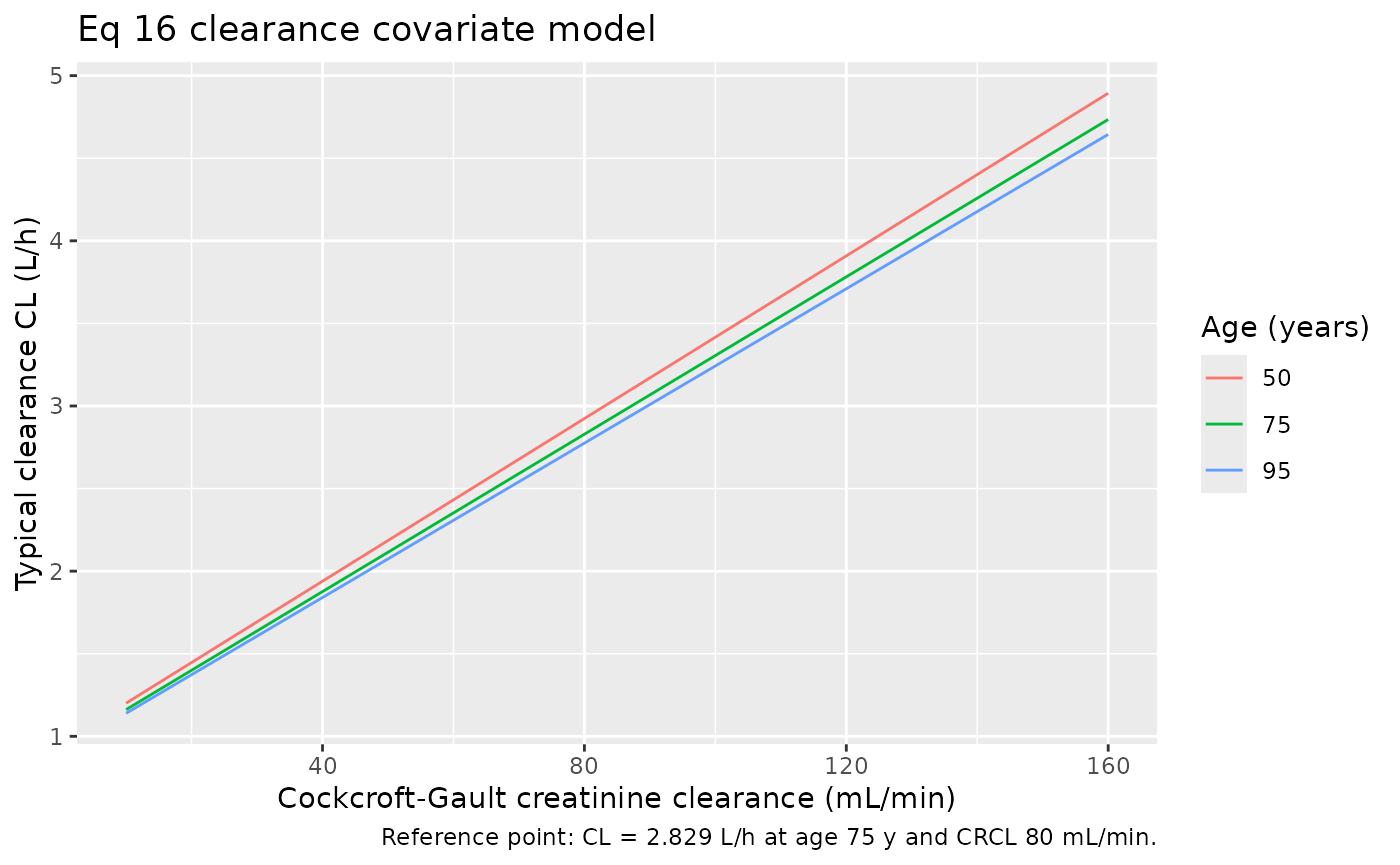
The full clearance covariate model (Ji 2017 Eq 16) is
CL = 2.829 * (1 + 0.00842 * (CLcr - 80)) * (75 / Age)^0.08143 * exp(eta1) (L/h)and the volume of distribution (Eq 17) is
V = 52.14 * exp(eta2) (L).
Virtual cohort
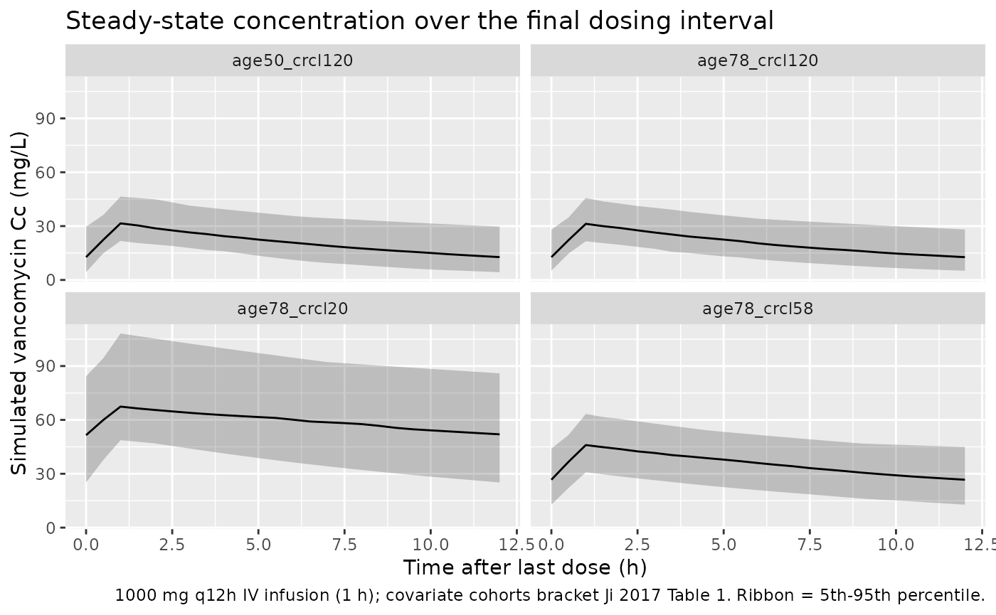
Original observed data are not publicly available. The cohort below covers four scenarios bracketing the paper’s covariate space: the typical model-building subject (median age, median CRCL), a good-renal-function subject, a poor-renal-function subject, and a younger high-clearance subject. All receive the studied regimen of 1000 mg every 12 h as a 1-hour IV infusion, simulated to steady state.
set.seed(20260527)

n_sub  <- 120L
tau    <- 12                      # dosing interval (h)
n_dose <- 14L                     # number of q12h doses -> steady state
dose_times <- seq(0, by = tau, length.out = n_dose)
last_dose  <- max(dose_times)     # 156 h
ss_end     <- last_dose + tau     # 168 h

# Observation grid: coarse over the whole horizon for the VPC, dense over the
# final (steady-state) dosing interval for NCA.
obs_times <- sort(unique(c(
  seq(0, ss_end, by = 3),
  seq(last_dose, ss_end, by = 0.5)
)))

build_arm <- function(label, age, crcl, id_offset) {
  ids <- id_offset + seq_len(n_sub)

  dose_rows <- tidyr::expand_grid(id = ids, time = dose_times) |>
    mutate(
      evid   = 1L,
      amt    = 1000,
      cmt    = "central",
      rate   = 1000 / 1,        # 1000 mg infused over 1 hour
      cohort = label,
      AGE    = age,
      CRCL   = crcl
    )

  obs_rows <- tidyr::expand_grid(id = ids, time = obs_times) |>
    mutate(
      evid   = 0L,
      amt    = 0,
      cmt    = NA_character_,
      rate   = 0,
      cohort = label,
      AGE    = age,
      CRCL   = crcl
    )

  bind_rows(dose_rows, obs_rows) |> arrange(id, time, desc(evid))
}

events <- bind_rows(
  build_arm("age78_crcl58",  78, 58,    0L),  # typical model-building subject
  build_arm("age78_crcl120", 78, 120, 120L),  # good renal function
  build_arm("age78_crcl20",  78, 20,  240L),  # poor renal function
  build_arm("age50_crcl120", 50, 120, 360L)   # younger, high clearance
)

stopifnot(!anyDuplicated(unique(events[, c("id", "time", "evid")])))
Simulation
mod <- readModelDb("Ji_2017_vancomycin")
sim <- rxode2::rxSolve(
  mod,
  events = events,
  keep   = c("cohort", "AGE", "CRCL")
) |> as.data.frame()
#> ℹ parameter labels from comments will be replaced by 'label()'
For the typical-value reproduction of Eq 16 (no between-subject variability), also simulate with the random effects zeroed:
mod_typical <- mod |> rxode2::zeroRe()
#> ℹ parameter labels from comments will be replaced by 'label()'
sim_typical <- rxode2::rxSolve(
  mod_typical,
  events = events,
  keep   = c("cohort", "AGE", "CRCL")
) |> as.data.frame()
#> ℹ omega/sigma items treated as zero: 'etalcl', 'etalvc'
#> Warning: multi-subject simulation without without 'omega'
Replicate published figures
Ji 2017 Figure 2 is a visual predictive check of trough concentrations and Figure 1 shows observed-vs-predicted goodness-of-fit clouds; neither is a per-subject concentration-time curve that can be reproduced directly. The block below summarises the simulated steady-state concentration-time profile for each covariate cohort, illustrating the renal- and age-dependent accumulation that drives the paper’s dose-individualisation analysis.
sim |>
  filter(time >= last_dose) |>
  mutate(tad = time - last_dose) |>
  group_by(cohort, tad) |>
  summarise(
    Q05 = quantile(Cc, 0.05, na.rm = TRUE),
    Q50 = quantile(Cc, 0.50, na.rm = TRUE),
    Q95 = quantile(Cc, 0.95, na.rm = TRUE),
    .groups = "drop"
  ) |>
  ggplot(aes(tad, Q50)) +
  geom_ribbon(aes(ymin = Q05, ymax = Q95), alpha = 0.25) +
  geom_line() +
  facet_wrap(~ cohort) +
  labs(
    x = "Time after last dose (h)",
    y = "Simulated vancomycin Cc (mg/L)",
    title = "Steady-state concentration over the final dosing interval",
    caption = "1000 mg q12h IV infusion (1 h); covariate cohorts bracket Ji 2017 Table 1. Ribbon = 5th-95th percentile."
  )
The clearance covariate relationships of Eq 16 (CL rises with creatinine clearance and falls with age) are reproduced directly from the packaged model’s typical-value clearance:
cov_grid <- tidyr::expand_grid(
  AGE  = c(50, 75, 95),
  CRCL = seq(10, 160, by = 10)
) |>
  mutate(CL = 2.829 * (1 + 0.00842 * (CRCL - 80)) * (75 / AGE)^0.08143)

ggplot(cov_grid, aes(CRCL, CL, colour = factor(AGE))) +
  geom_line() +
  labs(
    x = "Cockcroft-Gault creatinine clearance (mL/min)",
    y = "Typical clearance CL (L/h)",
    colour = "Age (years)",
    title = "Eq 16 clearance covariate model",
    caption = "Reference point: CL = 2.829 L/h at age 75 y and CRCL 80 mL/min."
  )
PKNCA validation
Ji 2017 does not publish an NCA table (Cmax / AUC); the model was
built on trough concentrations and used to drive a dose-targeting
simulation. The PKNCA block below characterises the steady-state
interval metrics (Cmax,ss, Tmax, Cmin/Ctrough = trough, Cavg, AUC0-tau)
over the final dosing interval for each covariate cohort, providing a
one-table audit of the simulated steady-state exposure. The treatment
grouping is cohort.
sim_nca <- sim |>
  filter(!is.na(Cc), time >= last_dose) |>
  select(id, time, Cc, cohort)

dose_df <- events |>
  filter(evid == 1, time == last_dose) |>
  select(id, time, amt, cohort)

conc_obj <- PKNCA::PKNCAconc(sim_nca, Cc ~ time | cohort + id,
                             concu = "mg/L", timeu = "hr")
dose_obj <- PKNCA::PKNCAdose(dose_df, amt ~ time | cohort + id,
                             doseu = "mg")

intervals <- data.frame(
  start   = last_dose,
  end     = ss_end,
  cmax    = TRUE,
  tmax    = TRUE,
  cmin    = TRUE,
  ctrough = TRUE,
  cav     = TRUE,
  auclast = TRUE
)

nca_res <- PKNCA::pk.nca(
  PKNCA::PKNCAdata(conc_obj, dose_obj, intervals = intervals)
)

nca_summary <- summary(nca_res)
knitr::kable(
  nca_summary,
  caption = "Simulated steady-state NCA parameters by covariate cohort (1000 mg q12h IV infusion, final dosing interval)."
)| Interval Start | Interval End | cohort | N | AUClast (hr*mg/L) | Cmax (mg/L) | Cmin (mg/L) | Tmax (hr) | Cav (mg/L) | Ctrough (mg/L) |
|---|---|---|---|---|---|---|---|---|---|
| 156 | 168 | age50_crcl120 | 120 | 247 [34.2] | 31.5 [24.0] | 12.1 [58.4] | 1.00 [1.00, 1.00] | 20.6 [34.2] | NC |
| 156 | 168 | age78_crcl120 | 120 | 248 [35.3] | 31.8 [24.4] | 11.9 [65.0] | 1.00 [1.00, 1.00] | 20.6 [35.3] | NC |
| 156 | 168 | age78_crcl20 | 120 | 709 [32.3] | 69.0 [27.3] | 49.7 [39.1] | 1.00 [1.00, 1.00] | 59.1 [32.3] | NC |
| 156 | 168 | age78_crcl58 | 120 | 417 [29.8] | 45.0 [23.8] | 25.8 [40.8] | 1.00 [1.00, 1.00] | 34.7 [29.8] | NC |
Comparison against published values
Ji 2017 reports no Cmax / AUC NCA table, so there is no published NCA row to compare against directly. The two checks below validate that the packaged model reproduces the paper’s structural parameter relationships.
# Typical clearance at the published reference point and at illustrative
# covariate values, computed (a) by hand from Eq 16 and (b) from the
# zero-random-effect simulation.
ref_check <- sim_typical |>
  # sim_typical retains per-subject cl/vc values inherited from the
  # preceding `sim` simulation's IIV state, so unique(cl) can return >1
  # value within a cohort. mean() collapses the per-id values back to
  # the typical-value cohort summary that this table is meant to show.
  group_by(cohort, AGE, CRCL) |>
  summarise(CL_model = mean(cl), V_model = mean(vc), .groups = "drop") |>
  mutate(
    CL_eq16 = 2.829 * (1 + 0.00842 * (CRCL - 80)) * (75 / AGE)^0.08143,
    V_eq17  = 52.14
  ) |>
  select(cohort, AGE, CRCL, CL_eq16, CL_model, V_eq17, V_model)

knitr::kable(
  ref_check,
  caption = "Typical CL (Eq 16) and V (Eq 17): hand-computed vs packaged-model values.",
  digits = 3
)| cohort | AGE | CRCL | CL_eq16 | CL_model | V_eq17 | V_model |
|---|---|---|---|---|---|---|
| age50_crcl120 | 50 | 120 | 3.909 | 3.909 | 52.14 | 52.14 |
| age78_crcl120 | 78 | 120 | 3.770 | 3.770 | 52.14 | 52.14 |
| age78_crcl20 | 78 | 20 | 1.395 | 1.395 | 52.14 | 52.14 |
| age78_crcl58 | 78 | 58 | 2.298 | 2.298 | 52.14 | 52.14 |
The packaged model returns CL = 2.829 L/h and V = 52.14 L at the reference subject (age 75 y, CRCL 80 mL/min), matching Ji 2017 Eq 16-17 / Table 3 exactly, and reproduces the hand-computed Eq 16 clearance at every cohort. Across the renal-function range the simulated steady-state troughs span roughly 14 mg/L (high clearance) to ~50 mg/L (CRCL 20 mL/min) for a fixed 1000 mg q12h regimen, consistent with the paper’s finding that renal function dominates vancomycin exposure and that dose individualisation is required to keep troughs within the 10-15 / 15-20 mg/L targets.
Assumptions and deviations
-
Age covariate coefficient (0.08143, not 0.8143). Ji
2017 Eq 16, the Abstract, and the Results text all state the age
exponent as 0.08143. Table 3 prints
theta Age_CL = 0.8143(RSE 53.68%) with bootstrap median0.8373– a 10x discrepancy. The packaged model uses 0.08143 because three independent statements (the model-defining equation, the abstract, and the Results narrative) agree on it, and only the single Table 3 cell (plus its bootstrap row) carries the larger value, which is a dropped-leading-zero typographical error. The directionality is also a cross-check: the paper states vancomycin excretion decreases as renal function diminishes with age, which(75/Age)^0.08143reproduces (CL falls as age rises above 75). Europe PMC (PMID 28836582) lists no erratum or corrigendum for this article. - Additive residual error units (mg/L, not ng/mL). Table 3 labels the additive residual row “Residual variability SD (ng/mL)” = 2.647, but the vancomycin concentration unit is mg/L throughout the paper (Table 1, LOQ 2.0 mg/L, target troughs in mg/L). An additive SD of 2.647 ng/mL (= 0.0026 mg/L) would be negligible and incompatible with the authors’ choice of a combined error model, whereas 2.647 mg/L is a sensible additive term near the 2.0 mg/L LOQ. The packaged model therefore treats 2.647 as mg/L; the “(ng/mL)” column label is read as a units typo.
-
One-compartment IV, no absorption compartment. The
Abstract and Results describe “first-order absorption” while the
Discussion says “zero-order absorption”, but vancomycin was given by
intravenous infusion and Table 3 estimates only CL and V (no absorption
rate constant). The drug is therefore dosed directly into the central
compartment as an IV infusion; no depot /
kais included, since none was estimated and inventing one is not supported by the source. -
IIV variances taken from the Results text. The
Results state the eta variances directly (“variances of 0.1051 and
0.083, respectively”) for CL and V; these go into
ini()as the omega values (etalcl ~ 0.1051,etalvc ~ 0.083). They reproduce the Table 3 “IIV (%)” rows on the square-root scale (sqrt(0.1051) = 32.4%; sqrt(0.083) = 28.8%). - Infusion duration. The paper records “continuous infusion of vancomycin (1000 mg q12 h)” with trough sampling before the next dose, i.e. intermittent q12h infusions. The infusion duration is not stated; the vignette assumes a 1-hour infusion (a common vancomycin practice and the same convention used in the Goti 2018 vancomycin vignette). The infusion duration has negligible effect on the modeled trough concentrations.
-
Year in the file name. The article was published
online in 2017 (DOI
10.1038/aps.2017.57) and in print in 2018 (Acta Pharmacol Sin 39(2):286-293). The model file / vignette name uses 2017 (online/DOI year); thereferencefield gives the full 2018 print citation. - Dose-individualisation supplements not used. The dosing-regimen tables (Tables S1-S4) referenced for the 10-15 and 15-20 mg/L trough targets are simulation outputs in the journal’s supplementary information and were not available when this model was built. They contain no model parameters (all final estimates are in Eq 16-17 and Table 3), so their absence does not affect the packaged model.
- Virtual-cohort demographics. Race / ethnicity beyond “Chinese adults” is not reported and is not a model covariate; the virtual cohort fixes age and CRCL per arm to illustrate the covariate effects rather than sampling the full joint demographic distribution.