Brentuximab vedotin ADC, MMAE payload and exposure-safety in ECHELON-1 (Suri 2019)
Source:vignettes/articles/Suri_2019_brentuximab.Rmd
Suri_2019_brentuximab.RmdSource and models
- Citation: Suri A, Mould DR, Song G, Collins GP, Endres CJ, Gomez-Navarro J, Venkatakrishnan K. Population Pharmacokinetic Modeling and Exposure-Response Assessment for the Antibody-Drug Conjugate Brentuximab Vedotin in Hodgkin’s Lymphoma in the Phase III ECHELON-1 Study. Clin Pharmacol Ther. 2019;106(6):1268-1279. doi:10.1002/cpt.1530. PMCID PMC6896233.
- Article (open access): https://doi.org/10.1002/cpt.1530
- PubMed Central: https://www.ncbi.nlm.nih.gov/pmc/articles/PMC6896233/
- Supporting Information (Figure S1, Tables S1-S4 and the Supplementary Supporting Information methods) is published with the open-access article (PMC6896233).
Suri 2019 reports the population PK of brentuximab vedotin (antibody-drug conjugate, ADC) and its payload monomethyl auristatin E (MMAE) in the A+AVD arm of the phase III ECHELON-1 study, and then relates the individual exposures to efficacy and safety. This package carries six files:
| File | Content |
|---|---|
Suri_2019_brentuximab |
Coupled ADC + MMAE popPK model (Table 2, Figure 1b) |
Suri_2019_brentuximab_pn |
Grade >= 2 peripheral neuropathy vs ADC AUC/time (Figure 4b) |
Suri_2019_brentuximab_fn_adc |
Febrile neutropenia vs ADC AUC/time and G-CSF (Figure 4c) |
Suri_2019_brentuximab_fn_mmae |
Febrile neutropenia vs MMAE AUC/time and G-CSF (Figure 4d) |
Suri_2019_brentuximab_neutropenia |
Grade >= 4 neutropenia vs MMAE AUC/time and G-CSF (Figure 4e) |
Suri_2019_brentuximab_teae |
Any grade >= 3 TEAE vs MMAE AUC/time and G-CSF (Figure 4f) |
The exposure-efficacy analysis (Cox model for modified PFS, Figure 4a) found no exposure relationship and reports no coefficients, and the non-significant exposure-safety pairs (Figure S1) were not retained, so neither is packaged.
Population
| Field | Value |
|---|---|
| Subjects | 661 |
| Age | 18-82 years (mean 38.7, SD 15.8) |
| Weight | 40.8-165.5 kg (mean 73.5, SD 18.0) |
| BSA | 1.3-2.8 m^2 (mean 1.8, SD 0.3) |
| Female | 43.1% |
| Disease | Previously untreated, histologically confirmed stage III or IV classical Hodgkin lymphoma (ECHELON-1, NCT01712490, A+AVD arm). |
| Dosing | Brentuximab vedotin 1.2 mg/kg as a 30-minute IV infusion on days 1 and 15 of 28-day cycles for up to 6 cycles, capped at 120 mg for patients above 100 kg, given within about 1 hour after doxorubicin, vinblastine and dacarbazine. |
| Observations | 33,164 concentration records (16,536 ADC, 16,628 MMAE) and 7,209 dosing records; 347 post-dose BLQ records excluded (42 ADC, 305 MMAE). |
Race: 84.3% White, 3.0% Black, 8.5% Asian, 2.7% other, 1.5% not reported. Mean (SD) albumin 39.1 (5.3) g/L, Cockcroft-Gault creatinine clearance 134.1 (45.4) mL/min and bilirubin 7.1 (5.4) umol/L (Suri 2019 Table 1).
Source trace
| Quantity | Value | Source |
|---|---|---|
| ADC structure: 3-compartment, zero-order input, first-order elimination | – | Results ‘ADC PK model’; Figure 1b |
| ADC CL, Vc, Q2, V2, Q3, V3 | 0.0615 L/h, 3.58 L, 0.113 L/h, 3.26 L, 0.0239 L/h, 15.7 L | Table 2 |
| ADC covariates: ALB on CL, BSA on CL, BSA on Vc, sex on Vc, BSA on V3 | -0.477, 1.1, 0.893, 0.934, 1.47 | Table 2 |
Covariate forms: (cov / population mean)^theta;
categorical theta^cov
|
– | Supplement, ‘Covariate model development’ |
| Reference values BSA / ALB / CrCl | 1.8 m^2 / 39.1 g/L / 134.1 mL/min | Table 1 means |
| ADC IIV (% CV): CL, Vc, V2, Q3, V3 | 19.8, 14.0, 25.5, 41.4, 77.7 | Table 2 |
| IIV scale: reported value = sqrt(omega^2) | omega^2 = (CV/100)^2 | Supplement, ‘Statistical model for inter-individual variation’ |
| MMAE structure: 2-compartment, formation via target binding and direct conversion through a lag compartment | – | Results ‘MMAE PK model’; Figure 1b |
| MMAE CL, Vc, Q, Vp | 1.45 L/h, 35.5 L, 13.2 L/h, 17.7 L | Table 2 |
| KD, FM, ALFM, Klag | 0.0376 1/h, 1 FIX, 2.35 1/h, 4.51 1/h | Table 2 |
| MMAE covariates: BSA, CrCl, ALB on CL | 1.04, 0.125, 0.0275 | Table 2 |
| MMAE IIV (% CV): CL, Vc, KD | 38.6, 68.6, 101.0 | Table 2 |
| Residual error (LTBS, log-scale SD) ADC / MMAE | 0.181 / 0.395 | Table 2; Supplement ‘Statistical model for residual variation’ |
| Molar units (amounts umol, concentrations uM) | – | Figure 3a, 3c axes |
Direct-conversion time function
1 - exp(-ALFM * tad)
|
– | Not printed; selected by reproducing Results (see below) |
Logistic model form
logit P = b0 + b1 * EXPOSURE + beta * X
|
– | Supplement, ‘Logistic regression model’ |
| Logistic coefficients | see each model file | Digitised from Figure 4b-f |
The MMAE direct-conversion term
Figure 1b names a fraction metabolised (FM, fixed to 1) and a rate
constant ALFM “to describe the decline in direct conversion of ADC to
MMAE following time after dose” (Table 2 footnote), but the paper prints
no equation. The literal reading, FM * exp(-ALFM * tad), is
the form used by the related Zhou 2025 pediatric model (whose control
stream is published), and the packaged Suri 2018 model uses it too. With
the ECHELON-1 estimate ALFM = 2.35 1/h, however, that form shuts direct
conversion off within about an hour of every dose. After the first dose
the target pool is depleted, so MMAE formation almost stops.
The paper gives three numbers that decide the question: the cycle-3 (dose 5) MMAE AUC of 10.0-11.3 ng*day/mL across weight bands, the 49% fall in MMAE exposure from dose 1 to dose 5, and the Figure 3d profile, in which MMAE accumulates cycle after cycle with a median peak near 1.3 ng/mL. The chunk below solves the reference patient (BSA 1.8 m^2, 73.5 kg, 1.2 mg/kg every 2 weeks) under both readings.
mw_adc  <- 153.4   # kDa, brentuximab vedotin
mw_mmae <- 718     # g/mol, MMAE

typ_events <- function(wt = 73.5, n_dose = 5, cov = list(BSA = 1.8, ALB = 39.1, CRCL = 134.1, SEXF = 0)) {
  dose_umol <- min(1.2 * wt, 120) / mw_adc
  dos <- data.frame(id = 1L, time = (seq_len(n_dose) - 1) * 336, evid = 1L, amt = dose_umol,
                    dur = 0.5, cmt = "central", dvid = NA_integer_)
  obs <- data.frame(id = 1L, time = seq(0, n_dose * 336, by = 1), evid = 0L, amt = 0,
                    dur = 0, cmt = NA_character_, dvid = 1L)
  out <- dplyr::bind_rows(dos, obs) |> dplyr::arrange(time, dplyr::desc(evid))
  for (nm in names(cov)) out[[nm]] <- cov[[nm]]
  out
}

auc_window <- function(t, y, a, b) {
  i <- t >= a & t <= b
  sum(diff(t[i]) * (head(y[i], -1) + tail(y[i], -1)) / 2)
}

ev_typ <- typ_events()
mod_literal <- mod_pk |> rxode2::model(fmt <- fm_mmae * exp(-alfm * tafd))
#> ℹ parameter labels from comments will be replaced by 'label()'

solve_typ <- function(m) {
  s <- as.data.frame(rxode2::rxSolve(m, events = ev_typ, omega = NA, sigma = NA,
                                     useLinCmt = FALSE, returnType = "data.frame"))
  tday <- s$time / 24
  data.frame(
    mmae_auc_d1 = auc_window(tday, s$Cc_mmae * mw_mmae, 0, 14),
    mmae_auc_d5 = auc_window(tday, s$Cc_mmae * mw_mmae, 56, 70),
    mmae_cmax_d5 = max(s$Cc_mmae[s$time >= 1344] * mw_mmae)
  )
}
forms <- dplyr::bind_rows(
  cbind(Form = "Packaged: FM * (1 - exp(-ALFM * tad))", solve_typ(mod_pk)),
  cbind(Form = "Literal: FM * exp(-ALFM * tad)", solve_typ(mod_literal))
) |>
  dplyr::mutate(ratio_d5_d1 = mmae_auc_d5 / mmae_auc_d1)
#> ℹ parameter labels from comments will be replaced by 'label()'

forms |>
  dplyr::rename(
    "MMAE AUC dose 1 (ng*day/mL)" = mmae_auc_d1,
    "MMAE AUC dose 5 (ng*day/mL)" = mmae_auc_d5,
    "MMAE Cmax dose 5 (ng/mL)" = mmae_cmax_d5,
    "Dose 5 / dose 1" = ratio_d5_d1
  ) |>
knitr::kable(digits = 3, caption = "Typical-value MMAE exposure under the two readings of the direct-conversion term. Published: dose-5 AUC 10.0-11.3 ng*day/mL; dose 5 / dose 1 = 0.51.")| Form | MMAE AUC dose 1 (ng*day/mL) | MMAE AUC dose 5 (ng*day/mL) | MMAE Cmax dose 5 (ng/mL) | Dose 5 / dose 1 |
|---|---|---|---|---|
| Packaged: FM * (1 - exp(-ALFM * tad)) | 21.069 | 11.320 | 1.645 | 0.537 |
| Literal: FM * exp(-ALFM * tad) | 12.474 | 0.263 | 0.061 | 0.021 |
# Deterministic typical-value solves: tight structural gates are appropriate.
stopifnot(
  forms$mmae_auc_d5[1] > 9, forms$mmae_auc_d5[1] < 13,
  abs(forms$ratio_d5_d1[1] - 0.51) < 0.08,
  forms$mmae_auc_d5[2] < 1   # the literal reading misses the published value ~40-fold
)
The packaged form reproduces the published cycle-3 MMAE AUC and the
49% decline from two independent numbers, with nothing tuned. The
literal form misses the cycle-3 AUC by a factor of about 40. The
complementary form also accounts for where the MMAE comes from: at
steady state, converting all eliminated ADC 1:1 to MMAE gives
dose / CL_MMAE = 11.9 ng*day/mL, which is essentially the
published value. The dose-1 excess comes from the one-time
target-binding pathway. A constant fraction (FM = 1 at every time)
cannot be distinguished numerically from the packaged form, because
1 - exp(-2.35 * tad) reaches 1 within about two hours. The
packaged form keeps ALFM, which the paper estimated with 0.2% SE, in the
model.
Virtual cohort
200 patients (a single A+AVD arm), with covariates drawn to match Suri 2019 Table 1. Height is not reported, so sex-specific heights are assumed and BSA is computed with the Mosteller formula; the covariates are otherwise drawn independently.
set.seed(20191201)
rxode2::rxSetSeed(20191201)
n_sub <- 200
clip <- function(x, lo, hi) pmin(pmax(x, lo), hi)
lnorm_draw <- function(n, mean, sd) {
  s2 <- log(1 + (sd / mean)^2)
  exp(rnorm(n, log(mean) - s2 / 2, sqrt(s2)))
}
cohort <- tibble::tibble(
  id   = seq_len(n_sub),
  SEXF = rbinom(n_sub, 1, 0.431),
  WT   = clip(ifelse(SEXF == 1, lnorm_draw(n_sub, 66, 15), lnorm_draw(n_sub, 79, 17)), 40.8, 165.5),
  HT   = ifelse(SEXF == 1, rnorm(n_sub, 163, 7), rnorm(n_sub, 176, 7)),
  BSA  = clip(sqrt(HT * WT / 3600), 1.3, 2.8),
  ALB  = clip(rnorm(n_sub, 39.1, 5.3), 17, 53),
  CRCL = clip(lnorm_draw(n_sub, 134.1, 45.4), 29.2, 476.7),
  GCSF = rbinom(n_sub, 1, 0.5),
  dose_mg = pmin(1.2 * WT, 120)
)
cohort |>
  dplyr::summarise(
    `Weight mean (kg)` = mean(WT), `BSA mean (m^2)` = mean(BSA),
    `Albumin mean (g/L)` = mean(ALB), `CrCl mean (mL/min)` = mean(CRCL),
    `Female (%)` = 100 * mean(SEXF)
  ) |>
knitr::kable(digits = 2, caption = "Simulated cohort summary; compare Suri 2019 Table 1 (73.5 kg, 1.8 m^2, 39.1 g/L, 134.1 mL/min, 43.1% female).")| Weight mean (kg) | BSA mean (m^2) | Albumin mean (g/L) | CrCl mean (mL/min) | Female (%) |
|---|---|---|---|---|
| 73.86 | 1.86 | 38.32 | 128.63 | 39.5 |
Each patient receives 1.2 mg/kg (capped at 120 mg) as a 30-minute infusion every 14 days for 12 doses (6 cycles), the ECHELON-1 schedule.
n_dose <- 12
dose_rows <- cohort |>
  tidyr::crossing(k = seq_len(n_dose) - 1) |>
  dplyr::transmute(id, time = k * 336, evid = 1L, amt = dose_mg / mw_adc, dur = 0.5,
                   cmt = "central", dvid = NA_integer_)
obs_rows <- cohort |>
  tidyr::crossing(time = seq(0, n_dose * 336, by = 4)) |>
  dplyr::transmute(id, time, evid = 0L, amt = 0, dur = 0, cmt = NA_character_, dvid = 1L)
events <- dplyr::bind_rows(dose_rows, obs_rows) |>
  dplyr::left_join(dplyr::select(cohort, id, SEXF, BSA, ALB, CRCL), by = "id") |>
  dplyr::arrange(id, time, dplyr::desc(evid))

sim <- as.data.frame(rxode2::rxSolve(mod_pk, events = events, useLinCmt = FALSE,
                                     returnType = "data.frame")) |>
  dplyr::mutate(time_d = time / 24, adc_ugml = Cc * mw_adc, mmae_ngml = Cc_mmae * mw_mmae)
Replicating Figure 3b and 3d
sim |>
  dplyr::filter(time_d <= 70) |>
  tidyr::pivot_longer(c(adc_ugml, mmae_ngml), names_to = "analyte", values_to = "conc") |>
  dplyr::mutate(analyte = dplyr::recode(analyte, adc_ugml = "ADC (ug/mL)", mmae_ngml = "MMAE (ng/mL)")) |>
  dplyr::group_by(analyte, time_d) |>
  dplyr::summarise(med = median(conc), lo = quantile(conc, 0.025), hi = quantile(conc, 0.975), .groups = "drop") |>
  ggplot(aes(time_d, med)) +
  geom_ribbon(aes(ymin = lo, ymax = hi), fill = "grey75") +
  geom_line(colour = "firebrick") +
  scale_y_log10() +
  facet_wrap(~analyte, scales = "free_y") +
  labs(x = "Days since first dose", y = "Concentration") +
  theme_bw()
#> Warning in scale_y_log10(): log-10 transformation introduced infinite values.
#> log-10 transformation introduced infinite values.
#> log-10 transformation introduced infinite values.
#> log-10 transformation introduced infinite values.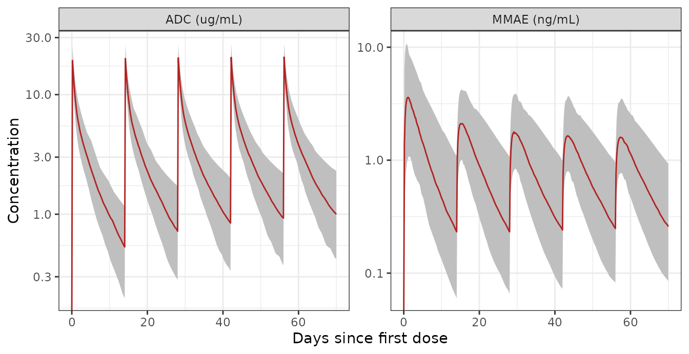
Replicates Figure 3b (ADC) and Figure 3d (MMAE) of Suri 2019: simulated median (line) and 95% prediction interval (band) over the first five doses of 1.2 mg/kg every 2 weeks.
As in the published panels, the median ADC peak is about 20 ug/mL with no visible accumulation of the peaks. The MMAE peak is highest after dose 1 and settles to a lower, repeating profile from dose 2 onwards.
PKNCA validation
AUC over the first dosing interval (dose 1, days 0-14) and over cycle 3 (dose 5, days 56-70), plus the whole 12-dose course (days 0-168) for the time-averaged exposure used by the exposure-response models.
arm_lbl <- "A+AVD, BV 1.2 mg/kg Q2W"
dose_nca <- cohort |>
  tidyr::crossing(k = seq_len(n_dose) - 1) |>
  dplyr::transmute(id, time_d = k * 14, dose = dose_mg, arm = arm_lbl)
intervals <- data.frame(start = c(0, 56, 0), end = c(14, 70, 168), auclast = TRUE)

run_nca <- function(conc_col) {
  conc <- sim |>
    dplyr::filter(!is.na(.data[[conc_col]])) |>
    dplyr::transmute(id, time_d, conc = .data[[conc_col]], arm = arm_lbl)
  o_conc <- PKNCA::PKNCAconc(conc, conc ~ time_d | arm + id)
  o_dose <- PKNCA::PKNCAdose(dose_nca, dose ~ time_d | arm + id)
  res <- PKNCA::pk.nca(PKNCA::PKNCAdata(o_conc, o_dose, intervals = intervals))
  as.data.frame(res$result) |>
    dplyr::filter(PPTESTCD == "auclast") |>
    dplyr::mutate(window = paste0(start, "-", end)) |>
    dplyr::select(id, window, PPORRES) |>
    tidyr::pivot_wider(names_from = window, values_from = PPORRES)
}
auc_adc  <- run_nca("adc_ugml")  |> dplyr::rename(adc_d1 = `0-14`, adc_d5 = `56-70`, adc_all = `0-168`)
auc_mmae <- run_nca("mmae_ngml") |> dplyr::rename(mmae_d1 = `0-14`, mmae_d5 = `56-70`, mmae_all = `0-168`)
exposure <- cohort |>
  dplyr::left_join(auc_adc, by = "id") |>
  dplyr::left_join(auc_mmae, by = "id") |>
  dplyr::mutate(
    AUC_BV_ADC  = adc_all / n_dose,   # time-averaged, per 14-day interval
    AUC_BV_MMAE = mmae_all / n_dose,
    wt_band   = cut(WT, c(0, 61, 71, 83, 100, Inf), right = FALSE,
                    labels = c("<61 kg", "61-<71 kg", "71-<83 kg", "83-100 kg", ">100 kg")),
    alb_band  = cut(ALB, c(0, 37, 43, Inf), right = FALSE, labels = c("<37 g/L", "37-<43 g/L", ">=43 g/L")),
    crcl_band = cut(CRCL, c(0, 90, Inf), right = FALSE, labels = c("<90 mL/min", ">=90 mL/min"))
  )
Comparison against published exposures
Suri 2019 quotes subgroup cycle-3 AUCs (Results, Figure 2), the ADC accumulation from cycle 1 to cycle 3, and the MMAE decline from dose 1 to dose 5.
sub_long <- dplyr::bind_rows(
  exposure |> dplyr::filter(wt_band == "<61 kg") |> dplyr::mutate(subgroup = "Weight <61 kg"),
  exposure |> dplyr::filter(wt_band == "83-100 kg") |> dplyr::mutate(subgroup = "Weight 83-100 kg"),
  exposure |> dplyr::filter(alb_band == "<37 g/L") |> dplyr::mutate(subgroup = "Albumin <37 g/L"),
  exposure |> dplyr::filter(alb_band == ">=43 g/L") |> dplyr::mutate(subgroup = "Albumin >=43 g/L"),
  exposure |> dplyr::filter(crcl_band == ">=90 mL/min") |> dplyr::mutate(subgroup = "CrCl >=90 mL/min")
)
sim_sub <- dplyr::bind_rows(
  sub_long |> dplyr::transmute(subgroup, PPTESTCD = "auclast", PPORRES = adc_d5, analyte = "ADC (ug*day/mL)"),
  sub_long |> dplyr::transmute(subgroup, PPTESTCD = "auclast", PPORRES = mmae_d5, analyte = "MMAE (ng*day/mL)")
) |>
  dplyr::mutate(group = paste(analyte, "-", subgroup)) |>
  dplyr::select(group, PPTESTCD, PPORRES)
ref_sub <- tibble::tribble(
  ~group,                                    ~auclast,
  "ADC (ug*day/mL) - Weight <61 kg",         48.8,
  "ADC (ug*day/mL) - Weight 83-100 kg",      63.6,
  "ADC (ug*day/mL) - Albumin <37 g/L",       49.5,
  "ADC (ug*day/mL) - Albumin >=43 g/L",      59.6,
  "MMAE (ng*day/mL) - Weight <61 kg",        10.0,
  "MMAE (ng*day/mL) - Weight 83-100 kg",     11.3,
  "MMAE (ng*day/mL) - CrCl >=90 mL/min",     11.3
)
cmp <- nlmixr2lib::ncaComparisonTable(sim_sub, ref_sub, by = "group",
                                      units = c(auclast = "per unit shown"))
knitr::kable(cmp, caption = "Cycle-3 (dose 5, days 56-70) AUC: simulated subgroup medians vs Suri 2019 Results / Figure 2.")| NCA parameter | group | Reference | Simulated | % diff |
|---|---|---|---|---|
| AUClast (per unit shown) | ADC (ug*day/mL) - Weight <61 kg | 48.8 | 42.4 | -13.2% |
| AUClast (per unit shown) | ADC (ug*day/mL) - Weight 83-100 kg | 63.6 | 52.6 | -17.3% |
| AUClast (per unit shown) | ADC (ug*day/mL) - Albumin <37 g/L | 49.5 | 48.3 | -2.3% |
| AUClast (per unit shown) | ADC (ug*day/mL) - Albumin >=43 g/L | 59.6 | 52.5 | -11.9% |
| AUClast (per unit shown) | MMAE (ng*day/mL) - Weight <61 kg | 10 | 8.97 | -10.3% |
| AUClast (per unit shown) | MMAE (ng*day/mL) - Weight 83-100 kg | 11.3 | 13.3 | +17.7% |
| AUClast (per unit shown) | MMAE (ng*day/mL) - CrCl >=90 mL/min | 11.3 | 11.5 | +1.3% |
ratios <- exposure |>
  dplyr::summarise(adc_accum = median(adc_d5 / adc_d1), mmae_decline = median(mmae_d5 / mmae_d1))
knitr::kable(
  data.frame(
    Quantity = c("ADC AUC dose 5 / dose 1", "MMAE AUC dose 5 / dose 1"),
    Published = c(1.27, 0.51),
    Simulated = c(ratios$adc_accum, ratios$mmae_decline)
  ),
  digits = 2, caption = "Accumulation (Results: ADC 1.27-fold between cycles 1 and 3; MMAE exposure 49% lower at dose 5 than dose 1)."
)| Quantity | Published | Simulated |
|---|---|---|
| ADC AUC dose 5 / dose 1 | 1.27 | 1.22 |
| MMAE AUC dose 5 / dose 1 | 0.51 | 0.58 |
# Cohort medians: centre-of-distribution gates only (not cohort extremes).
stopifnot(
  abs(median(exposure$adc_d5) / 58 - 1) < 0.2,
  abs(median(exposure$mmae_d5) / 11 - 1) < 0.25,
  abs(ratios$adc_accum - 1.27) < 0.15,
  abs(ratios$mmae_decline - 0.51) < 0.12
)
The subgroup AUCs land within 18% of the published values and carry the same body-size, albumin and renal trends. The simulated ADC values run about 2-17% low. To separate the model from the cohort, the chunk below solves representative typical patients at the published covariate means, with no random effects:
typ_adc_d5 <- function(wt, bsa) {
  ev <- typ_events(wt = wt, cov = list(BSA = bsa, ALB = 39.1, CRCL = 134.1, SEXF = 0))
  s <- as.data.frame(rxode2::rxSolve(mod_pk, events = ev, omega = NA, sigma = NA,
                                     useLinCmt = FALSE, returnType = "data.frame"))
  auc_window(s$time / 24, s$Cc * mw_adc, 56, 70)
}
adc_typ <- data.frame(
  Patient = c("55 kg, BSA 1.60 m^2 (weight <61 kg)", "90 kg, BSA 2.05 m^2 (weight 83-100 kg)"),
  Published = c(48.8, 63.6),
  Typical = c(typ_adc_d5(55, 1.60), typ_adc_d5(90, 2.05))
)
knitr::kable(adc_typ, digits = 1, caption = "Typical-value cycle-3 ADC AUC (ug*day/mL) for representative patients vs Suri 2019 Results.")| Patient | Published | Typical |
|---|---|---|
| 55 kg, BSA 1.60 m^2 (weight <61 kg) | 48.8 | 48.1 |
| 90 kg, BSA 2.05 m^2 (weight 83-100 kg) | 63.6 | 59.2 |
At the typical value the model is within 1-7% of the published
subgroup AUCs. Dose 5 is about 94% of the way to steady state, and the
published values sit close to the steady-state dose / CL.
The remaining cohort shortfall comes from the virtual cohort: its mean
BSA (1.86 m^2) is above the published 1.8 m^2, which raises ADC
clearance, and its covariates are drawn independently, whereas in
ECHELON-1 weight, BSA, sex and creatinine clearance are correlated.
Time-averaged exposure vs the Figure 4a quartiles
Figure 4a divides the efficacy analysis set at ADC AUC/time quartile
boundaries of 50.4, 58.2 and 65.8 ug*day/mL. The simulated whole-course
time-averaged AUC (AUC_BV_ADC, per 14-day interval) falls
about 14% below these boundaries. That is a larger gap than the cycle-3
comparison above, because the whole-course average also contains the
first, pre-accumulation cycle. How the source defined the averaging
window for efficacy (to progression or censoring) cannot be reproduced
exactly, so this is a level check only.
q_sim <- quantile(exposure$AUC_BV_ADC, c(0.25, 0.5, 0.75))
knitr::kable(
  data.frame(Quartile = c("25th", "50th", "75th"), Published = c(50.4, 58.2, 65.8), Simulated = as.numeric(q_sim)),
  digits = 1, caption = "ADC AUC/time quartile boundaries (ug*day/mL): Suri 2019 Figure 4a vs simulated."
)| Quartile | Published | Simulated |
|---|---|---|
| 25th | 50.4 | 42.1 |
| 50th | 58.2 | 50.3 |
| 75th | 65.8 | 55.9 |
Sex effect on ADC central volume
The Results state that Vc was about 20% lower in females than in males. That figure includes the lower BSA of females; the 0.934 sex multiplier alone is a 6.6% reduction.
vc_by_sex <- sim |>
  dplyr::distinct(id, v1_adc) |>
  dplyr::left_join(dplyr::select(cohort, id, SEXF), by = "id") |>
  dplyr::group_by(SEXF) |>
  dplyr::summarise(vc = median(v1_adc), .groups = "drop")
vc_ratio <- vc_by_sex$vc[vc_by_sex$SEXF == 1] / vc_by_sex$vc[vc_by_sex$SEXF == 0]
vc_ratio
#> [1] 0.8242976
stopifnot(vc_ratio > 0.7, vc_ratio < 0.92)
Exposure-safety models
Digitised coefficients reproduce Figure 4
The coefficients were digitised from Figure 4b-f: each fitted line was traced at 400 dpi over about 900 pixel columns and fitted with the supplement’s logistic form (linear exposure, additive G-CSF term on the logit). For every G-CSF panel the no-G-CSF and G-CSF curves, fitted separately, gave slopes within 1% of each other, which confirms the shared-slope form. The joint fits have root-mean-square residuals of 0.07-0.26 percentage points. The table checks the packaged models against probabilities read directly off the traced curves.
solve_prob <- function(model, output, auc_col, auc, gcsf = NULL) {
  ev <- data.frame(id = seq_along(auc), time = 0, amt = 0, evid = 0L)
  ev[[auc_col]] <- auc
  if (!is.null(gcsf)) ev$CONMED_GCSF <- gcsf
  as.data.frame(rxode2::rxSolve(model, events = ev, returnType = "data.frame"))[[output]]
}
digitised <- tibble::tribble(
  ~panel, ~gcsf, ~auc, ~p_fig,
  "4b PN (ADC)",          NA, 30, 0.059, "4b PN (ADC)",          NA, 60, 0.105, "4b PN (ADC)",          NA, 90, 0.202,
  "4c FN (ADC)",           0, 30, 0.110, "4c FN (ADC)",           0, 60, 0.206, "4c FN (ADC)",           0, 90, 0.355,
  "4c FN (ADC)",           1, 30, 0.051, "4c FN (ADC)",           1, 60, 0.103, "4c FN (ADC)",           1, 90, 0.196,
  "4d FN (MMAE)",          0,  5, 0.097, "4d FN (MMAE)",          0, 25, 0.489, "4d FN (MMAE)",          1, 25, 0.281,
  "4e Neutropenia (MMAE)", 0,  5, 0.340, "4e Neutropenia (MMAE)", 0, 35, 0.598, "4e Neutropenia (MMAE)", 1, 35, 0.323,
  "4f TEAE (MMAE)",        0,  5, 0.821, "4f TEAE (MMAE)",        1,  5, 0.470, "4f TEAE (MMAE)",        1, 35, 0.809
)
er_map <- list(
  "4b PN (ADC)"           = list(m = mod_pn,   out = "prob_peripheral_neuropathy_grade2", col = "AUC_BV_ADC"),
  "4c FN (ADC)"           = list(m = mod_fna,  out = "prob_febrile_neutropenia",          col = "AUC_BV_ADC"),
  "4d FN (MMAE)"          = list(m = mod_fnm,  out = "prob_febrile_neutropenia",          col = "AUC_BV_MMAE"),
  "4e Neutropenia (MMAE)" = list(m = mod_neut, out = "prob_neutropenia_grade4",           col = "AUC_BV_MMAE"),
  "4f TEAE (MMAE)"        = list(m = mod_teae, out = "prob_teae_grade3",                  col = "AUC_BV_MMAE")
)
digitised$p_model <- vapply(seq_len(nrow(digitised)), function(i) {
  e <- er_map[[digitised$panel[i]]]
  g <- if (is.na(digitised$gcsf[i])) NULL else digitised$gcsf[i]
  solve_prob(e$m, e$out, e$col, digitised$auc[i], g)
}, numeric(1))
digitised |>
  dplyr::rename(Panel = panel, `G-CSF` = gcsf, AUC = auc, `Figure 4 (traced)` = p_fig, `Packaged model` = p_model) |>
knitr::kable(digits = 3, caption = "Event probability read from the traced Figure 4 curves vs the packaged models.")| Panel | G-CSF | AUC | Figure 4 (traced) | Packaged model |
|---|---|---|---|---|
| 4b PN (ADC) | NA | 30 | 0.059 | 0.058 |
| 4b PN (ADC) | NA | 60 | 0.105 | 0.110 |
| 4b PN (ADC) | NA | 90 | 0.202 | 0.200 |
| 4c FN (ADC) | 0 | 30 | 0.110 | 0.109 |
| 4c FN (ADC) | 0 | 60 | 0.206 | 0.206 |
| 4c FN (ADC) | 0 | 90 | 0.355 | 0.355 |
| 4c FN (ADC) | 1 | 30 | 0.051 | 0.052 |
| 4c FN (ADC) | 1 | 60 | 0.103 | 0.103 |
| 4c FN (ADC) | 1 | 90 | 0.196 | 0.196 |
| 4d FN (MMAE) | 0 | 5 | 0.097 | 0.097 |
| 4d FN (MMAE) | 0 | 25 | 0.489 | 0.488 |
| 4d FN (MMAE) | 1 | 25 | 0.281 | 0.281 |
| 4e Neutropenia (MMAE) | 0 | 5 | 0.340 | 0.340 |
| 4e Neutropenia (MMAE) | 0 | 35 | 0.598 | 0.598 |
| 4e Neutropenia (MMAE) | 1 | 35 | 0.323 | 0.323 |
| 4f TEAE (MMAE) | 0 | 5 | 0.821 | 0.821 |
| 4f TEAE (MMAE) | 1 | 5 | 0.470 | 0.469 |
| 4f TEAE (MMAE) | 1 | 35 | 0.809 | 0.808 |
Cross-check against the stated G-CSF effect
The Results report that G-CSF primary prophylaxis “significantly reduced the probability of FN, grade >= 4 neutropenia, and grade >= 3 TEAE by 55-81%”. This number was not used in the digitisation. The odds reductions implied by the digitised G-CSF coefficients are:
gcsf_coef <- c(
  "FN (ADC)"               = rxode2::rxode(mod_fna)$theta[["e_conmed_gcsf_fn"]],
  "FN (MMAE)"              = rxode2::rxode(mod_fnm)$theta[["e_conmed_gcsf_fn"]],
  "Grade >= 4 neutropenia" = rxode2::rxode(mod_neut)$theta[["e_conmed_gcsf_neut"]],
  "Grade >= 3 TEAE"        = rxode2::rxode(mod_teae)$theta[["e_conmed_gcsf_teae"]]
)
red <- 100 * (1 - exp(gcsf_coef))
knitr::kable(data.frame(Endpoint = names(red), `Odds reduction (%)` = red, check.names = FALSE),
digits = 1, row.names = FALSE)| Endpoint | Odds reduction (%) |
|---|---|
| FN (ADC) | 55.7 |
| FN (MMAE) | 59.0 |
| Grade >= 4 neutropenia | 68.0 |
| Grade >= 3 TEAE | 80.7 |
The range, 56-81%, matches the stated 55-81% at both ends.
Replicating Figure 4b-f
grid_adc  <- seq(20, 110, by = 1)
grid_mmae <- seq(2, 41, by = 0.5)
curves <- dplyr::bind_rows(lapply(names(er_map), function(p) {
  e <- er_map[[p]]
  g <- if (e$col == "AUC_BV_ADC") grid_adc else grid_mmae
  if (p == "4b PN (ADC)") {
    return(tibble::tibble(panel = p, auc = g, gcsf = "No", p = solve_prob(e$m, e$out, e$col, g)))
  }
  dplyr::bind_rows(
    tibble::tibble(panel = p, auc = g, gcsf = "No", p = solve_prob(e$m, e$out, e$col, g, 0)),
    tibble::tibble(panel = p, auc = g, gcsf = "Yes", p = solve_prob(e$m, e$out, e$col, g, 1))
  )
}))
#> Warning: multi-subject simulation without without 'omega'
#> Warning: multi-subject simulation without without 'omega'
#> Warning: multi-subject simulation without without 'omega'
#> Warning: multi-subject simulation without without 'omega'
#> Warning: multi-subject simulation without without 'omega'
#> Warning: multi-subject simulation without without 'omega'
#> Warning: multi-subject simulation without without 'omega'
#> Warning: multi-subject simulation without without 'omega'
#> Warning: multi-subject simulation without without 'omega'
ggplot(curves, aes(auc, p, colour = gcsf)) +
  geom_line(linewidth = 0.9) +
  scale_colour_manual(values = c(No = "firebrick", Yes = "navy"), name = "Prophylactic G-CSF") +
  facet_wrap(~panel, scales = "free_x") +
  coord_cartesian(ylim = c(0, 1)) +
  labs(x = "Time-averaged AUC (ADC ug*day/mL; MMAE ng*day/mL)", y = "Probability of event") +
  theme_bw()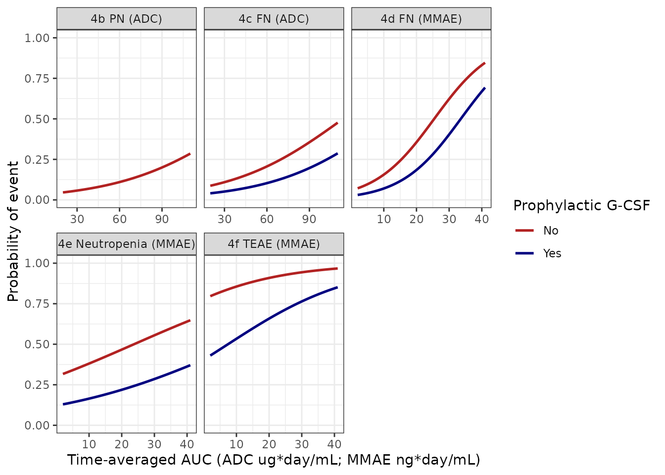
Replicates Figure 4b-f of Suri 2019: probability of each safety event against time-averaged ADC or MMAE AUC, without (red) and with (blue) G-CSF primary prophylaxis.
Coupling the PK and exposure-safety models
Using the simulated cohort’s time-averaged exposures (half assigned to G-CSF prophylaxis), the ADC-driven febrile neutropenia model predicts the incidences below. ECHELON-1 observed 21% without and 11% with primary G-CSF prophylaxis in the A+AVD arm (Suri 2019 Discussion, citing Connors 2018). The published models average exposure only up to each patient’s event, while this simulation averages over the whole course, so the comparison checks level, not precision.
fn_pred <- exposure |>
  dplyr::mutate(
    p_fn_adc  = solve_prob(mod_fna, "prob_febrile_neutropenia", "AUC_BV_ADC", AUC_BV_ADC, GCSF),
    p_fn_mmae = solve_prob(mod_fnm, "prob_febrile_neutropenia", "AUC_BV_MMAE", AUC_BV_MMAE, GCSF)
  ) |>
  dplyr::group_by(GCSF) |>
  dplyr::summarise(`FN via ADC model` = mean(p_fn_adc), `FN via MMAE model` = mean(p_fn_mmae), .groups = "drop") |>
  dplyr::mutate(Observed = ifelse(GCSF == 1, 0.11, 0.21))
#> Warning: There were 2 warnings in `dplyr::mutate()`.
#> The first warning was:
#> ℹ In argument: `p_fn_adc = solve_prob(...)`.
#> Caused by warning:
#> ! multi-subject simulation without without 'omega'
#> ℹ Run `dplyr::last_dplyr_warnings()` to see the 1 remaining warning.
fn_pred |>
  dplyr::rename(`Primary G-CSF` = GCSF) |>
knitr::kable(digits = 3, caption = "Mean predicted febrile-neutropenia probability vs observed ECHELON-1 incidence.")| Primary G-CSF | FN via ADC model | FN via MMAE model | Observed |
|---|---|---|---|
| 0 | 0.170 | 0.226 | 0.21 |
| 1 | 0.088 | 0.108 | 0.11 |
Assumptions and deviations
-
Direct-conversion time function (structural). Suri
2019 prints no equation for the ADC-to-MMAE direct flux. The packaged
FM * (1 - exp(-ALFM * tad))was selected because it reproduces the paper’s own cycle-3 MMAE AUC, its 49% dose-1-to-dose-5 decline and the Figure 3d profile. The literal reading of the prose,FM * exp(-ALFM * tad), misses the AUC about 40-fold (see “The MMAE direct-conversion term”). Nothing was tuned. A reviewer who obtains the ECHELON-1 control stream should confirm the form. -
Molar units. The paper does not state dosing units,
but Figure 3a/3c plot both analytes in uM. The target-binding flux
KD * Target * ADCdepends on the amount unit, and umol reproduces the published exposures. Molecular weights used for conversion: ADC 153.4 kDa, MMAE 718 g/mol. - IIV scale. The supplement reports each IIV as sqrt(omega^2), so omega^2 = (CV/100)^2 rather than log(1 + CV^2).
-
Residual error. LTBS with a homoscedastic additive
log-scale error, so
lnorm()with the reported CV used as the log-scale SD. - BSA effect on peripheral volume 2. Table 2 and the supplement place the BSA effect on ‘peripheral volume 2’ (V3 in Table 2’s own naming), while the Results prose says ‘first peripheral volume (V2)’. The table and supplement are followed; the Zhou 2025 control stream from the same group also carries BSA on V3.
- Reference BSA 1.8 m^2. Table 1 prints the mean BSA to one decimal only.
- Sex coding. 0.934 is applied to females (SEXF = 1), following the supplement’s example that the reference subgroup (males) is coded 0. With the lower BSA of females, this gives the ~20% lower female Vc the Results state.
-
Exposure-safety coefficients are digitised. No
coefficient is tabulated. Values were traced from Figure 4b-f; the
known-answer and G-CSF checks above bound their accuracy.
AUC_BV_ADC/AUC_BV_MMAEare time-averaged AUCs expressed per 14-day interval, which is the scale of the Figure 4 axes. The source averages up to each patient’s event; this vignette averages over the whole course. -
Placeholder residual on probabilities. Each
logistic model carries a
fixed(0.001)additive residual only so rxode2 accepts an endpoint; the source likelihood is Bernoulli. - Virtual cohort. Height and the covariate correlations are not reported. Sex-specific heights and weights were assumed, and the covariates were drawn independently. G-CSF prophylaxis was assigned to half the cohort for illustration.
- Errata. No erratum or corrigendum for Suri 2019 was found in the Europe PMC record or on the journal page.