Trastuzumab deruxtecan in vitro and mouse xenograft QSP (Vasalou 2024)
Source:vignettes/articles/Vasalou_2024_trastuzumabDeruxtecan.Rmd
Vasalou_2024_trastuzumabDeruxtecan.RmdModel and source
- Citation: Vasalou C, Proia TA, Kazlauskas L, Przybyla A, Sung M, Mamidi S, Maratea K, Griffin M, Sargeant R, Urosevic J, Rosenbaum AI, Yuan J, Aluri KC, Ramsden D, Hariparsad N, Jones RDO, Mettetal JT. Quantitative evaluation of trastuzumab deruxtecan pharmacokinetics and pharmacodynamics in mouse models of varying degrees of HER2 expression. CPT Pharmacometrics Syst Pharmacol. 2024;13(6):994. doi:10.1002/psp4.13133.
- Article: https://doi.org/10.1002/psp4.13133 (open access, PMC11179703)
- Appendix S1 (model equations 2-27, Tables S1-S3) and Appendix S3 (NONMEM control streams for the DAR, plasma and tumor fits) are open access.
The paper characterises trastuzumab deruxtecan (T-DXd) and its released topoisomerase-I-inhibitor payload DXd in four human tumor xenografts whose HER2 density spans three orders of magnitude, and builds two mechanistic models. The package ships both, sharing this article:
-
Vasalou_2024_trastuzumabDeruxtecan_invitro_qsp: the cellular disposition model fitted to medium and intracellular DXd in NCI-N87 and NCI-H322 cell monolayers (Appendix S1 Eqs 2-9, Table S1). Time in hours. -
Vasalou_2024_trastuzumabDeruxtecan_mouse_qsp: plasma total antibody, intact T-DXd and released DXd, a Krogh-cylinder tumor disposition model with HER2 binding and trafficking, and an indirect-response model of tumor gamma-H2AX (Eqs 10-27, Table S2). Time in days.
Both are deterministic. The in-vivo model was fitted naive-pooled with proportional residual errors whose estimates are not reported, and the in-vitro model reports no residual error, so neither file carries IIV or residual error.
mod_iv <- readModelDb("Vasalou_2024_trastuzumabDeruxtecan_invitro_qsp")
mod_mouse <- readModelDb("Vasalou_2024_trastuzumabDeruxtecan_mouse_qsp")
Population
- In vitro. NCI-N87 (gastric carcinoma, HER2-high) and NCI-H322 (non-small-cell lung carcinoma) monolayers in 6-well plates: 1.5 mL phenol-free RPMI per well, 1.2e6 (N87) or 2e6 (H322) cells, three replicate wells per condition and time point. Continuous exposure to 10 ug/mL T-DXd, datopotamab deruxtecan (Dato-DXd), or DAR4 / DAR8 isotype-control ADCs for up to 48 h; 50 ng/mL unconjugated DXd continuously or for 2 h followed by washout (N87 only). Appendix S1, ‘In-vitro experimental design’.
- Mouse. Male nude (NCI-N87), female nude (JIMT-1), male NOD-SCID (Capan-1) and female NOD-SCID (MDA-MB-468) mice, 5-8 weeks old, carrying subcutaneous tumors of about 300 mm^3 at dosing. A single IV dose of 1 mg/kg (NCI-N87, MDA-MB-468) or 10 mg/kg (all four) T-DXd; three mice per group per time point to 14 days (Methods, Figure 1c). HER2 receptors per cell: NCI-N87 3.5e6 (IHC 3+), JIMT-1 3.8e5 (2+), Capan-1 ~2e4 (2+, literature), MDA-MB-468 4.8e3 (IHC 0) (Results, Figure 1b).
str(mod_mouse()$population)
#> List of 9
#>  $ species      : chr "mouse (male/female nude and NOD-SCID, human tumor xenografts)"
#>  $ n_subjects   : int NA
#>  $ n_studies    : int 1
#>  $ age_range    : chr "5-8 weeks at study start"
#>  $ weight_range : chr "20 g assumed for tumor-volume scaling (Table S2)"
#>  $ disease_state: chr "Subcutaneous human tumor xenografts of differing HER2 expression, approximately 300 mm^3 at dosing: NCI-N87 gas"| __truncated__
#>  $ dose_range   : chr "Single IV dose of 1 mg/kg (NCI-N87, MDA-MB-468) or 10 mg/kg (all four xenografts) trastuzumab deruxtecan"
#>  $ regions      : chr "Preclinical (Axis Bioservices, UK)"
#>  $ notes        : chr "Sparse terminal sampling: three mice per treatment group per time point up to 14 days. Plasma total antibody, i"| __truncated__
Source trace
Every ini() value carries an in-file comment naming its
source. The equations map as follows.
| Model element | Source location |
|---|---|
In-vitro medium ADC (media_adc) |
Appendix S1 Eq 2, multiplied through by MV so the state is an amount |
Bound, endosomal ADC per cell (cell_bound_adc,
cell_endo_adc) |
Eqs 3-4 |
Intracellular and medium DXd (cell_dxd,
media_dxd) |
Eqs 5-6 |
| DAR decay | Eqs 7 and 11 |
Cmedia_dxd, Ccell_dxd
|
Eqs 8-9 |
| In-vitro parameters (N cell, MV, KD, koff, kint, kdegrad, Ag cell, kdec, kinD = keffD) | Table S1, T-DXd / N87 column |
| Plasma total antibody 2-compartment model with tumor exchange | Eqs 12-13, 17-18; control stream
DADT(1)-DADT(2)
|
| Released DXd in plasma | Eqs 14, 19; control stream DADT(5) (QDrug fixed to 0,
so one compartment) |
Intact T-DXd Cc = Cc_tab * DAR / DAR0
|
Eq 16; control stream IPRE for
CMT = 3
|
| Tumor unbound, bound, endosomal antibody | Eqs 20-22; control stream
DADT(8)-DADT(10)
|
| Tumor intracellular, extracellular DXd and their sum | Eqs 23-25; control stream
DADT(11)-DADT(12), DXDT
|
HER2 concentration ag from receptors per cell |
Eq 26; control stream Ttotal
|
| Tumor radius and tumor volume per body weight | Table S2 (R_tumor 0.41 cm, TV 0.015 L/kg);
control stream Rtumor, TV_BW
|
| Plasma PK values (CL, Vc, Q, Vp, kdec, CL_Drug, V_Drug) | Table S2; full precision from the fixed $THETA of
Figure5D_TumorFits.txt
|
| Tumor transport, binding and trafficking values | Table S2 |
| Cell-line receptors per cell and kint | Table S2; control stream IF (TYPE.EQ.n) blocks |
| Re-estimated JIMT-1 kint 0.14 1/day | Table S2 footnote; Results, Figure 5d dashed line |
| gamma-H2AX indirect response (kinp = koutp, PDmax, IC50_PD) | Eq 27; Table S2 |
Derived quantities against Table S2
Table S2 lists a few values the authors calculated rather than fitted. The model recomputes them from its inputs, so they are exact checks of the unit handling.
cell_lines <- tibble::tribble(
  ~xenograft,   ~CELLLINE_CAPAN1, ~CELLLINE_JIMT1, ~CELLLINE_MDAMB468, ~ag_tableS2,
  "NCI-N87",    0,                0,               0,                  1937,
  "Capan-1",    1,                0,               0,                  11,
  "JIMT-1",     0,                1,               0,                  210,
  "MDA-MB-468", 0,                0,               1,                  2.7
)

derived <- bind_rows(lapply(seq_len(nrow(cell_lines)), function(i) {
  cl <- cell_lines[i, ]
  s <- rxode2::rxSolve(
    mod_mouse,
    rxode2::et(0),
    params = unlist(cl[, c("CELLLINE_CAPAN1", "CELLLINE_JIMT1", "CELLLINE_MDAMB468")]),
    returnType = "data.frame"
  )
  tibble::tibble(
    xenograft = cl$xenograft,
    ag_model = s$ag[1],
    ag_tableS2 = cl$ag_tableS2,
    kint_model = s$kint[1],
    rtumor_cm = s$rtumor[1],
    tvbw_L_per_kg = s$tvbw[1],
    kon_per_nM_day = s$kon[1]
  )
}))
knitr::kable(derived, digits = 3)| xenograft | ag_model | ag_tableS2 | kint_model | rtumor_cm | tvbw_L_per_kg | kon_per_nM_day |
|---|---|---|---|---|---|---|
| NCI-N87 | 1937.019 | 1937.0 | 0.360 | 0.415 | 0.015 | 7.044 |
| Capan-1 | 11.069 | 11.0 | 2.770 | 0.415 | 0.015 | 7.044 |
| JIMT-1 | 210.305 | 210.0 | 0.140 | 0.415 | 0.015 | 7.044 |
| MDA-MB-468 | 2.673 | 2.7 | 4.158 | 0.415 | 0.015 | 7.044 |
stopifnot(
  all(abs(derived$ag_model / derived$ag_tableS2 - 1) < 0.02),
  all(abs(derived$rtumor_cm - 0.41) < 0.01),
  all(abs(derived$tvbw_L_per_kg - 0.015) < 1e-9),
  all(abs(derived$kon_per_nM_day - 7) < 0.1)
)
The receptor-derived HER2 concentrations reproduce Table S2’s 1937, 11, 210 and 2.7 nM; the tumor radius is 0.41 cm, the tumor volume per body weight 0.015 L/kg, and kon = koff / KD = 7 1/(nM day).
In vitro model: Figure 4
Each in-vitro condition uses the same structure with the Table S1 values for that ADC and cell line. The model’s defaults are T-DXd in N87 cells; the other conditions override them. Isotype-control ADCs have no target, so their antigen count is zero, and the deconjugation rate is the cell-line value of Table S1 for every ADC.
# Moles added to 1.5 mL of medium
mw_tdxd <- 153700 # g/mol, Appendix S1 'Data Analysis and PK metrics'
mw_mab <- 150000 # g/mol, used for Dato-DXd and the isotype controls
mw_dxd <- 493.5 # g/mol
adc_nmol <- function(mw) 10e-6 * 1.5 / mw * 1e9 # 10 ug/mL
dxd_nmol <- 50e-9 * 1.5 / mw_dxd * 1e9 # 50 ng/mL

n87 <- c(ncell = 1.2e6, lkdec = log(5.9e-5))
h322 <- c(ncell = 2e6, lkdec = log(4e-4))
dato <- function(ag, kint) {
  c(kd = 0.74, lkoff = log(0.26), ag_cell = ag, lkint = log(kint), dar0 = 4)
}
iso <- function(dar) c(ag_cell = 0, dar0 = dar)

iv_scen <- list(
  list(line = "N87", agent = "DAR4 isotype", p = c(n87, iso(4)), mw = mw_mab, cmt = "media_adc"),
  list(line = "N87", agent = "DAR8 isotype", p = c(n87, iso(8)), mw = mw_mab, cmt = "media_adc"),
  list(line = "N87", agent = "Dato-DXd", p = c(n87, dato(2e5, 0.37)), mw = mw_mab, cmt = "media_adc"),
  list(line = "N87", agent = "T-DXd", p = n87, mw = mw_tdxd, cmt = "media_adc"),
  list(line = "N87", agent = "DXd continuous", p = n87, mw = NA, cmt = "media_dxd"),
  list(line = "N87", agent = "DXd 2 h washout", p = n87, mw = NA, cmt = "media_dxd"),
  list(line = "H322", agent = "DAR4 isotype", p = c(h322, iso(4)), mw = mw_mab, cmt = "media_adc"),
  list(line = "H322", agent = "DAR8 isotype", p = c(h322, iso(8)), mw = mw_mab, cmt = "media_adc"),
  list(line = "H322", agent = "Dato-DXd", p = c(h322, dato(507145, 0.13)), mw = mw_mab, cmt = "media_adc")
)

iv_times <- sort(unique(c(seq(0, 48, by = 0.1), 1 / 3, 2 + 1 / 6)))
sim_iv <- bind_rows(lapply(iv_scen, function(sc) {
  amt <- if (is.na(sc$mw)) dxd_nmol else adc_nmol(sc$mw)
  ev <- rxode2::et(amt = amt, cmt = sc$cmt)
  if (sc$agent == "DXd 2 h washout") {
    # Medium replaced with drug-free medium at 2 h
    ev <- rxode2::et(ev, time = 2, amt = 0, cmt = "media_dxd", evid = 5)
  }
  ev <- rxode2::et(ev, iv_times, cmt = "media_dxd")
  s <- rxode2::rxSolve(mod_iv, ev, params = sc$p, returnType = "data.frame")
  tibble::tibble(
    line = sc$line, agent = sc$agent, time = s$time,
    Media = s$Cmedia_dxd, Intracellular = s$Ccell_dxd
  )
}))
sim_iv |>
  pivot_longer(c(Media, Intracellular), names_to = "space", values_to = "conc") |>
  filter(conc > 1e-4) |>
  ggplot(aes(time, conc, colour = space)) +
  geom_line() +
  scale_y_log10() +
  facet_grid(line ~ agent) +
  scale_colour_manual(values = c(Intracellular = "red", Media = "black")) +
  labs(
    x = "Time (h)", y = "DXd (nM)", colour = NULL,
    caption = "Replicates Figure 4 of Vasalou 2024 (typical-value model predictions)."
  ) +
  theme_bw() +
  theme(legend.position = "bottom", strip.text.x = element_text(size = 7))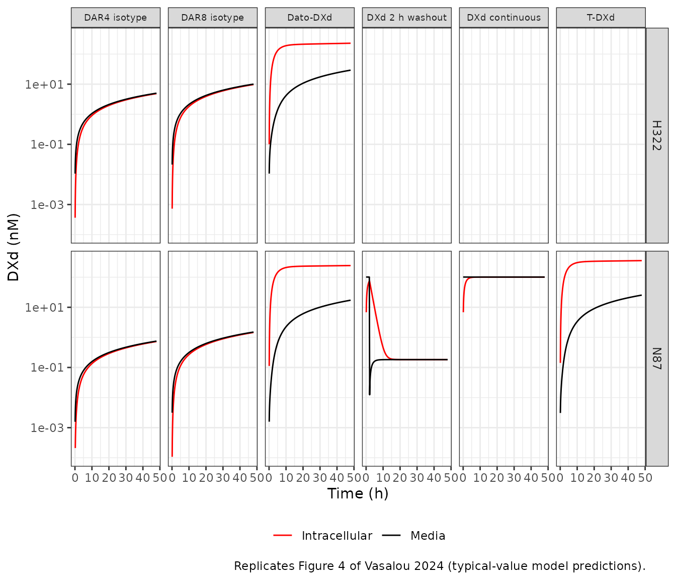
The paper’s qualitative findings hold. For T-DXd and Dato-DXd in N87 cells, intracellular DXd exceeds medium DXd by more than ten-fold at 48 h. For Dato-DXd in H322 cells the model gives about eight-fold, a little short of the more than ten-fold the Results text describes for the data. For the isotype controls, which have no receptor-mediated delivery, intracellular DXd only tracks the medium DXd that deconjugation releases, at slightly below one-to-one. Unconjugated DXd equilibrates across the membrane within a few hours and washes out at the same rate.
iv_48 <- sim_iv |>
  filter(abs(time - 48) < 1e-8) |>
  mutate(ratio = Intracellular / Media)
knitr::kable(iv_48, digits = 3)| line | agent | time | Media | Intracellular | ratio |
|---|---|---|---|---|---|
| N87 | DAR4 isotype | 48 | 0.751 | 0.729 | 0.970 |
| N87 | DAR8 isotype | 48 | 1.503 | 1.458 | 0.970 |
| N87 | Dato-DXd | 48 | 17.185 | 243.454 | 14.167 |
| N87 | T-DXd | 48 | 25.389 | 355.142 | 13.988 |
| N87 | DXd continuous | 48 | 101.075 | 101.075 | 1.000 |
| N87 | DXd 2 h washout | 48 | 0.183 | 0.183 | 1.000 |
| H322 | DAR4 isotype | 48 | 5.004 | 4.857 | 0.971 |
| H322 | DAR8 isotype | 48 | 10.007 | 9.715 | 0.971 |
| H322 | Dato-DXd | 48 | 29.179 | 229.068 | 7.851 |
ratio_at <- function(l, a) iv_48$ratio[iv_48$line == l & iv_48$agent == a]
stopifnot(
  ratio_at("N87", "T-DXd") > 10,
  ratio_at("N87", "Dato-DXd") > 10,
  ratio_at("H322", "Dato-DXd") > 5,
  ratio_at("N87", "DAR8 isotype") < 1,
  # kinD = keffD with no binding: free DXd equilibrates (ratio ~ 1)
  abs(ratio_at("N87", "DXd continuous") - 1) < 0.01
)
Mouse model: plasma and tumor time courses (Figure 5)
Doses are converted to molar units with the T-DXd molecular weight,
153.7 kDa (10 mg/kg = 65.1 nmol/kg). The cell line is selected with the
CELLLINE_* indicators; all zero is NCI-N87.
arms <- tibble::tribble(
  ~treatment,              ~xenograft,   ~dose_mgkg, ~CELLLINE_CAPAN1, ~CELLLINE_JIMT1, ~CELLLINE_MDAMB468,
  "NCI-N87 1 mg/kg",       "NCI-N87",    1,          0,                0,               0,
  "NCI-N87 10 mg/kg",      "NCI-N87",    10,         0,                0,               0,
  "Capan-1 10 mg/kg",      "Capan-1",    10,         1,                0,               0,
  "JIMT-1 10 mg/kg",       "JIMT-1",     10,         0,                1,               0,
  "MDA-MB-468 1 mg/kg",    "MDA-MB-468", 1,          0,                0,               1,
  "MDA-MB-468 10 mg/kg",   "MDA-MB-468", 10,         0,                0,               1
) |>
  mutate(id = row_number(), dose_nmolkg = dose_mgkg * 1e-3 / mw_tdxd * 1e9)

obs_times <- sort(unique(c(seq(0, 1, by = 0.02), seq(1, 14, by = 0.1))))
events <- bind_rows(
  arms |> transmute(id, time = 0, amt = dose_nmolkg, evid = 1L, cmt = "central_tab"),
  tidyr::expand_grid(id = arms$id, time = obs_times) |>
    mutate(amt = 0, evid = 0L, cmt = "central_tab")
) |>
  left_join(arms |> select(id, starts_with("CELLLINE_")), by = "id") |>
  arrange(id, time, desc(evid))

sim_mouse <- rxode2::rxSolve(mod_mouse, events, returnType = "data.frame") |>
  left_join(arms |> select(id, treatment, xenograft, dose_mgkg), by = "id")

# Plasma-only fitting stage (Eqs 12-14): an enormous body weight makes the
# tumor volume per body weight, and so the tumor's pull on plasma, negligible.
sim_plasma_stage <- rxode2::rxSolve(
  mod_mouse, events,
  params = c(bw = 1e9), returnType = "data.frame"
) |>
  left_join(arms |> select(id, treatment, xenograft, dose_mgkg), by = "id")
The authors fitted the model in stages. The plasma parameters were estimated with the plasma-only equations (Appendix S1 Eqs 12-14), and Figure 5a-c show that stage: one plasma profile per dose, identical across xenografts. The tumor model was then added with the plasma parameters fixed, and its equations (Eqs 17-19, and the deposited tumor-fit control stream) let antibody and DXd move between plasma and tumor. The packaged model is the final, integrated one. In NCI-N87, with 3.5e6 HER2 receptors per cell, the tumor takes up enough antibody to lower plasma total antibody visibly; in the low-HER2 lines the effect is small. The figure shows both: solid lines are the integrated model, dashed lines the plasma-only stage.
# Plasma-only stage: total antibody AUC0-inf must equal dose / CL_mAb
mb_stage <- sim_plasma_stage |> filter(treatment == "MDA-MB-468 10 mg/kg")
auc_14 <- sum(diff(mb_stage$time) *
  (head(mb_stage$Cc_tab, -1) + tail(mb_stage$Cc_tab, -1)) / 2)
# Two-compartment tail beyond 14 days: last concentration / terminal slope
lambda_z <- -diff(log(tail(mb_stage$Cc_tab, 2))) / diff(tail(mb_stage$time, 2))
auc_inf <- auc_14 + tail(mb_stage$Cc_tab, 1) / lambda_z
auc_closed <- arms$dose_nmolkg[arms$treatment == "MDA-MB-468 10 mg/kg"] / 0.02378
c(numerical = auc_inf, closed_form = auc_closed)
#>   numerical closed_form
#>    2736.143    2735.989
stopifnot(abs(auc_inf / auc_closed - 1) < 0.01)
fig5_long <- function(d, stage) {
  d |>
    transmute(
      xenograft, dose = paste(dose_mgkg, "mg/kg"), time,
      `1. Total mAb plasma` = Cc_tab / 1000,
      `2. ADC plasma` = Cc / 1000,
      `3. Released DXd plasma` = Cc_dxd / 1000,
      `4. Released DXd tumor` = Ctumor_dxd / 1000
    ) |>
    pivot_longer(-c(xenograft, dose, time), names_to = "analyte", values_to = "conc_uM") |>
    mutate(stage = stage)
}
bind_rows(
  fig5_long(sim_mouse, "Integrated model"),
  fig5_long(sim_plasma_stage, "Plasma-only stage") |>
    filter(analyte != "4. Released DXd tumor")
) |>
  filter(conc_uM > 1e-5) |>
  ggplot(aes(time, conc_uM, colour = dose, linetype = stage)) +
  geom_line() +
  scale_linetype_manual(values = c("Integrated model" = "solid", "Plasma-only stage" = "dashed")) +
  scale_y_log10() +
  facet_grid(xenograft ~ analyte) +
  scale_colour_manual(values = c("1 mg/kg" = "orchid", "10 mg/kg" = "navy")) +
  labs(
    x = "Time (days)", y = "Concentration (uM)", colour = NULL, linetype = NULL,
    caption = "Replicates Figure 5a-d of Vasalou 2024 (JIMT-1 with the re-estimated kint)."
  ) +
  theme_bw() +
  theme(legend.position = "bottom", strip.text = element_text(size = 7))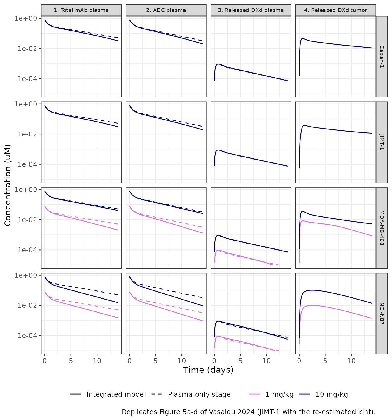
ggplot(sim_mouse, aes(time, gh2ax_pct, colour = paste(dose_mgkg, "mg/kg"))) +
  geom_line() +
  scale_y_log10(limits = c(10, 1000)) +
  facet_wrap(~xenograft) +
  scale_colour_manual(values = c("1 mg/kg" = "orchid", "10 mg/kg" = "navy")) +
  labs(
    x = "Time (days)", y = "% gamma-H2AX of vehicle", colour = NULL,
    caption = "Replicates Figure 5e of Vasalou 2024."
  ) +
  theme_bw()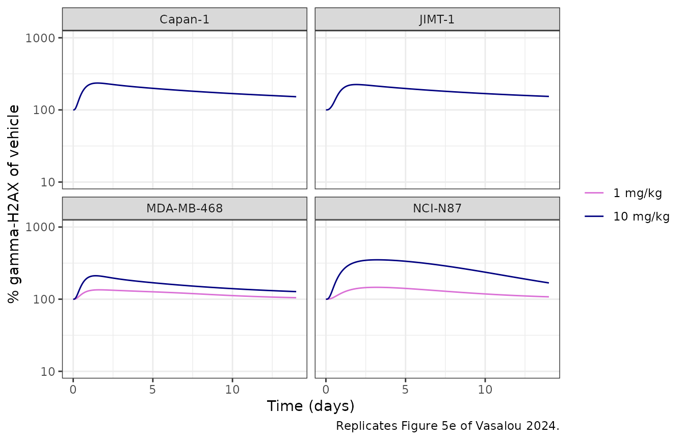
The predicted profiles have the shapes and magnitudes of the published fits: NCI-N87 tumor DXd peaks near 0.1 uM at 10 mg/kg, plasma DXd near 1 nM, and gamma-H2AX rises with a delay of about three days to roughly three-fold of vehicle in NCI-N87, with smaller increases in the lower-HER2 lines.
pd_peak <- sim_mouse |>
  filter(dose_mgkg == 10) |>
  group_by(xenograft) |>
  summarise(
    peak_pct = max(gh2ax_pct),
    tpeak_day = time[which.max(gh2ax_pct)],
    tumor_dxd_cmax_nM = max(Ctumor_dxd),
    .groups = "drop"
  )
knitr::kable(pd_peak, digits = 2)| xenograft | peak_pct | tpeak_day | tumor_dxd_cmax_nM |
|---|---|---|---|
| Capan-1 | 235.70 | 1.5 | 45.61 |
| JIMT-1 | 224.80 | 1.9 | 38.00 |
| MDA-MB-468 | 211.21 | 1.4 | 36.03 |
| NCI-N87 | 351.28 | 3.2 | 100.07 |
pk_n87 <- pd_peak[pd_peak$xenograft == "NCI-N87", ]
stopifnot(
  # Baseline gamma-H2AX is kinp / koutp = 1, i.e. 100 % of vehicle
  all(abs(sim_mouse$gh2ax_pct[sim_mouse$time == 0] - 100) < 1e-6),
  pk_n87$peak_pct > 250, pk_n87$peak_pct < 450,
  pk_n87$tpeak_day > 2, pk_n87$tpeak_day < 5,
  # The highest-HER2 line has the largest response
  pk_n87$peak_pct == max(pd_peak$peak_pct)
)
PKNCA validation against Tables 1 and 2
Table 1 reports NCA of the mean plasma profiles (Phoenix sparse sampling); Table 2 the released-DXd AUC and Cmax in tumor at 10 mg/kg. The same parameters are computed from the typical-value predictions over the 14-day study window, one profile per arm.
pknca_plasma <- function(conc_col, analyte) {
  conc <- sim_mouse |>
    transmute(id, treatment, time, conc = .data[[conc_col]] / 1000) |>
    filter(!is.na(conc))
  dose <- arms |> transmute(id, treatment, time = 0, dose = dose_nmolkg / 1000)
  o_conc <- PKNCA::PKNCAconc(conc, conc ~ time | treatment + id)
  o_dose <- PKNCA::PKNCAdose(dose, dose ~ time | treatment + id, route = "intravascular")
  intervals <- data.frame(
    start = 0, end = Inf, aucinf.obs = TRUE, half.life = TRUE,
    cl.obs = TRUE, vss.obs = TRUE
  )
  res <- PKNCA::pk.nca(PKNCA::PKNCAdata(o_conc, o_dose, intervals = intervals))
  as.data.frame(res) |>
    filter(PPTESTCD %in% c("aucinf.obs", "half.life", "cl.obs", "vss.obs")) |>
    mutate(
      # dose in umol/kg and concentration in uM give L/kg; Table 1 reports mL/kg
      PPORRES = ifelse(PPTESTCD %in% c("cl.obs", "vss.obs"), PPORRES * 1000, PPORRES),
      analyte = analyte
    ) |>
    select(treatment, analyte, PPTESTCD, PPORRES)
}

nca_plasma <- bind_rows(
  pknca_plasma("Cc_tab", "Total antibody"),
  pknca_plasma("Cc", "T-DXd")
) |>
  filter(treatment != "MDA-MB-468 1 mg/kg") |>
  mutate(treatment = paste(treatment, analyte, sep = ", ")) |>
  select(-analyte)

# Table 1 (total antibody / T-DXd); MDA-MB-468 1 mg/kg was not analysed
table1 <- tibble::tribble(
  ~treatment,           ~aucinf.obs, ~half.life, ~cl.obs, ~vss.obs,
  "Capan-1 10 mg/kg, Total antibody",    2.32, 1.5, 27.9, 77.4,
  "Capan-1 10 mg/kg, T-DXd",             1.96, 1.5, 33.2, 79.5,
  "JIMT-1 10 mg/kg, Total antibody",     3.88, 3.8, 16.7, 86.1,
  "JIMT-1 10 mg/kg, T-DXd",              2.75, 3.4, 23.7, 105.5,
  "MDA-MB-468 10 mg/kg, Total antibody", 3.00, 3.5, 21.6, 97.3,
  "MDA-MB-468 10 mg/kg, T-DXd",          2.48, 3.2, 26.2, 99.6,
  "NCI-N87 1 mg/kg, Total antibody",     0.23, 3.2, 27.5, 117.5,
  "NCI-N87 1 mg/kg, T-DXd",              0.20, 2.9, 32.5, 123.7,
  "NCI-N87 10 mg/kg, Total antibody",    2.89, 5.3, 22.4, 153.2,
  "NCI-N87 10 mg/kg, T-DXd",             2.40, 4.5, 26.6, 146.3
)

cmp_plasma <- nlmixr2lib::ncaComparisonTable(
  simulated = nca_plasma,
  reference = table1,
  by = "treatment",
  units = c(aucinf.obs = "uM*day", half.life = "day", cl.obs = "mL/kg/day", vss.obs = "mL/kg"),
  tolerance_pct = 20
)
knitr::kable(
  cmp_plasma,
  caption = "Plasma NCA vs. Table 1. * differs from the published value by >20%."
)| NCA parameter | treatment | Reference | Simulated | % diff |
|---|---|---|---|---|
| AUC0-∞ (obs) (uM*day) | Capan-1 10 mg/kg, Total antibody | 2.32 | 2.26 | -2.7% |
| AUC0-∞ (obs) (uM*day) | Capan-1 10 mg/kg, T-DXd | 1.96 | 1.92 | -2.2% |
| AUC0-∞ (obs) (uM*day) | JIMT-1 10 mg/kg, Total antibody | 3.88 | 2.16 | -44.2%* |
| AUC0-∞ (obs) (uM*day) | JIMT-1 10 mg/kg, T-DXd | 2.75 | 1.84 | -33.1%* |
| AUC0-∞ (obs) (uM*day) | MDA-MB-468 10 mg/kg, Total antibody | 3 | 2.45 | -18.4% |
| AUC0-∞ (obs) (uM*day) | MDA-MB-468 10 mg/kg, T-DXd | 2.48 | 2.03 | -17.9% |
| AUC0-∞ (obs) (uM*day) | NCI-N87 1 mg/kg, Total antibody | 0.23 | 0.163 | -29.1%* |
| AUC0-∞ (obs) (uM*day) | NCI-N87 1 mg/kg, T-DXd | 0.2 | 0.143 | -28.4%* |
| AUC0-∞ (obs) (uM*day) | NCI-N87 10 mg/kg, Total antibody | 2.89 | 1.63 | -43.6%* |
| AUC0-∞ (obs) (uM*day) | NCI-N87 10 mg/kg, T-DXd | 2.4 | 1.43 | -40.3%* |
| t½ (day) | Capan-1 10 mg/kg, Total antibody | 1.5 | 3.48 | +132.3%* |
| t½ (day) | Capan-1 10 mg/kg, T-DXd | 1.5 | 2.99 | +99.4%* |
| t½ (day) | JIMT-1 10 mg/kg, Total antibody | 3.8 | 3.47 | -8.8% |
| t½ (day) | JIMT-1 10 mg/kg, T-DXd | 3.4 | 2.98 | -12.4% |
| t½ (day) | MDA-MB-468 10 mg/kg, Total antibody | 3.5 | 4.51 | +28.9%* |
| t½ (day) | MDA-MB-468 10 mg/kg, T-DXd | 3.2 | 3.75 | +17.3% |
| t½ (day) | NCI-N87 1 mg/kg, Total antibody | 3.2 | 3.23 | +0.9% |
| t½ (day) | NCI-N87 1 mg/kg, T-DXd | 2.9 | 2.78 | -4.0% |
| t½ (day) | NCI-N87 10 mg/kg, Total antibody | 5.3 | 3.23 | -39.1%* |
| t½ (day) | NCI-N87 10 mg/kg, T-DXd | 4.5 | 2.78 | -38.1%* |
| CL/F (mL/kg/day) | Capan-1 10 mg/kg, Total antibody | 27.9 | 28.8 | +3.3% |
| CL/F (mL/kg/day) | Capan-1 10 mg/kg, T-DXd | 33.2 | 33.9 | +2.2% |
| CL/F (mL/kg/day) | JIMT-1 10 mg/kg, Total antibody | 16.7 | 30.1 | +80.1%* |
| CL/F (mL/kg/day) | JIMT-1 10 mg/kg, T-DXd | 23.7 | 35.4 | +49.3%* |
| CL/F (mL/kg/day) | MDA-MB-468 10 mg/kg, Total antibody | 21.6 | 26.6 | +23.0%* |
| CL/F (mL/kg/day) | MDA-MB-468 10 mg/kg, T-DXd | 26.2 | 32 | +22.0%* |
| CL/F (mL/kg/day) | NCI-N87 1 mg/kg, Total antibody | 27.5 | 39.9 | +45.2%* |
| CL/F (mL/kg/day) | NCI-N87 1 mg/kg, T-DXd | 32.5 | 45.4 | +39.7%* |
| CL/F (mL/kg/day) | NCI-N87 10 mg/kg, Total antibody | 22.4 | 39.9 | +78.2%* |
| CL/F (mL/kg/day) | NCI-N87 10 mg/kg, T-DXd | 26.6 | 45.4 | +70.7%* |
| Vss/F (mL/kg) | Capan-1 10 mg/kg, Total antibody | 77.4 | 150 | +94.2%* |
| Vss/F (mL/kg) | Capan-1 10 mg/kg, T-DXd | 79.5 | 149 | +87.2%* |
| Vss/F (mL/kg) | JIMT-1 10 mg/kg, Total antibody | 86.1 | 156 | +81.2%* |
| Vss/F (mL/kg) | JIMT-1 10 mg/kg, T-DXd | 106 | 154 | +46.3%* |
| Vss/F (mL/kg) | MDA-MB-468 10 mg/kg, Total antibody | 97.3 | 161 | +66.0%* |
| Vss/F (mL/kg) | MDA-MB-468 10 mg/kg, T-DXd | 99.6 | 158 | +58.2%* |
| Vss/F (mL/kg) | NCI-N87 1 mg/kg, Total antibody | 118 | 163 | +38.9%* |
| Vss/F (mL/kg) | NCI-N87 1 mg/kg, T-DXd | 124 | 158 | +27.5%* |
| Vss/F (mL/kg) | NCI-N87 10 mg/kg, Total antibody | 153 | 163 | +6.6% |
| Vss/F (mL/kg) | NCI-N87 10 mg/kg, T-DXd | 146 | 158 | +7.8% |
conc_tumor <- sim_mouse |>
  filter(dose_mgkg == 10) |>
  transmute(id, treatment, time, conc = Ctumor_dxd) |>
  filter(!is.na(conc))
dose_tumor <- arms |>
  filter(dose_mgkg == 10) |>
  transmute(id, treatment, time = 0, dose = dose_nmolkg)
res_tumor <- PKNCA::pk.nca(PKNCA::PKNCAdata(
  PKNCA::PKNCAconc(conc_tumor, conc ~ time | treatment + id),
  PKNCA::PKNCAdose(dose_tumor, dose ~ time | treatment + id),
  intervals = data.frame(start = 0, end = Inf, cmax = TRUE, aucinf.obs = TRUE)
))

table2 <- tibble::tribble(
  ~treatment,            ~aucinf.obs, ~cmax,
  "Capan-1 10 mg/kg",    237.6,       39.3,
  "JIMT-1 10 mg/kg",     168.4,       19.4,
  "MDA-MB-468 10 mg/kg", 156.5,       31.8,
  "NCI-N87 10 mg/kg",    493.6,       74.2
)
cmp_tumor <- nlmixr2lib::ncaComparisonTable(
  simulated = res_tumor,
  reference = table2,
  by = "treatment",
  params = c("cmax", "aucinf.obs"),
  units = c(cmax = "nM", aucinf.obs = "nM*day"),
  tolerance_pct = 20
)
knitr::kable(
  cmp_tumor,
  caption = "Released DXd in tumor vs. Table 2. * differs from the published value by >20%."
)| NCA parameter | treatment | Reference | Simulated | % diff |
|---|---|---|---|---|
| Cmax (nM) | Capan-1 10 mg/kg | 39.3 | 45.6 | +16.0% |
| Cmax (nM) | JIMT-1 10 mg/kg | 19.4 | 38 | +95.9%* |
| Cmax (nM) | MDA-MB-468 10 mg/kg | 31.8 | 36 | +13.3% |
| Cmax (nM) | NCI-N87 10 mg/kg | 74.2 | 100 | +34.9%* |
| AUC0-∞ (obs) (nM*day) | Capan-1 10 mg/kg | 238 | 434 | +82.6%* |
| AUC0-∞ (obs) (nM*day) | JIMT-1 10 mg/kg | 168 | 455 | +170.3%* |
| AUC0-∞ (obs) (nM*day) | MDA-MB-468 10 mg/kg | 156 | 243 | +55.5%* |
| AUC0-∞ (obs) (nM*day) | NCI-N87 10 mg/kg | 494 | 833 | +68.8%* |
sim_res_tumor <- as.data.frame(res_tumor) |>
  filter(PPTESTCD == "aucinf.obs") |>
  arrange(desc(PPORRES))
stopifnot(
  # Tumor DXd exposure ranks with HER2 density at the top: NCI-N87 highest
  sim_res_tumor$treatment[1] == "NCI-N87 10 mg/kg"
)
The comparison is against non-compartmental summaries of sparse, terminal mean data, not against the model’s own predictions, so differences beyond 20% are expected where the published fit and the data part ways:
- One plasma parameter set for all arms. Table 1’s total-antibody AUC varies from 2.32 to 3.88 uMday across the 10 mg/kg arms; the model has a single set of plasma parameters, so it sits inside that range (dose / CL is 2.74 uMday before any tumor uptake) and misses the extremes, notably the high JIMT-1 AUC.
- NCI-N87 plasma. The integrated model gives NCI-N87 a lower AUC and a higher clearance than the other lines, because its HER2-rich tumor takes up antibody (Eq 17; see the dashed plasma-only lines in the figure above). The NCA of the data does not show this, and neither does Figure 5a, which plots the plasma-only stage. It is a property of the published integrated model, whose plasma parameters were fixed from the plasma-only stage, not a transcription error.
- Capan-1 half-life. The observed 1.5 days reflects the low 14-day samples that the paper attributes to sparse-sampling variability.
- Vss. The model’s steady-state volume, Vc + Vp = 164 mL/kg, is above the 77-153 mL/kg of Table 1; the NCA volumes come from a few mean concentrations per arm and differ by a factor of two between arms.
- Tumor DXd. The model reproduces the ordering of exposure, highest in NCI-N87, and Cmax within 20% for Capan-1 and MDA-MB-468. It overpredicts the tumor AUC in every line and the JIMT-1 Cmax, as the solid and dashed lines of Figure 5d also lie at or above most of the data after the first days.
No parameter was adjusted to improve these comparisons.
Assumptions and deviations
-
Cell-line selection. The authors’ NONMEM
TYPEcolumn (1 NCI-N87, 2 Capan-1, 3 JIMT-1, 4 MDA-MB-468) is decomposed into the binary indicatorsCELLLINE_CAPAN1,CELLLINE_JIMT1andCELLLINE_MDAMB468, with NCI-N87 as the all-zero reference; the maintainers registered thisCELLLINE_<NAME>family for the purpose. -
Integrated model, not the plasma-only stage. The
model file implements the final equations (Eqs 17-27), in which plasma
and tumor exchange antibody and DXd. The plasma-only fitting stage (Eqs
12-14), which Figure 5a-c plot, is recovered by setting
bwto a very large value, as this article does. - JIMT-1 internalization. The deposited tumor-fit control stream carries the literature JIMT-1 kint of 5.54 1/day; the model uses the re-estimated 0.14 1/day (Table S2 footnote), which the paper carried forward into the PD fit and plots as the dashed JIMT-1 line in Figure 5d.
- MDA-MB-468 receptors. 4830 per cell, from the control stream; Table S2 and Figure 1b round it to 4.8e3.
-
pi. The control stream uses
pi = 3.14for the tumor radius; the model uses R’spi, which changes the radius by under 0.02%. - Dose conversion. T-DXd doses are converted with the 153.7 kDa molecular weight the paper gives for the ADC. Dato-DXd and the isotype controls, whose molecular weights the paper does not give, use the 150 kDa it gives for the antibody.
- In-vitro conditions other than T-DXd / N87. These use the Table S1 overrides: Dato-DXd KD 0.74 nM, koff 0.26 1/h, DAR 4, receptors 2e5 (N87) and 507145 (H322), kint 0.37 and 0.13 1/h; N87 and H322 cell counts and deconjugation rates; zero antigen for the isotype controls. T-DXd in H322 is not simulated because Table S1 gives no internalization rate for it.
-
Washout. The 2 h DXd washout replaces the medium
DXd amount with zero at 2 h (
evid = 5); intracellular DXd is carried over. - No residual error. The NONMEM fits estimated proportional (and for tumor DXd also additive) residual errors whose estimates are not reported; the in- vitro model reports none. Both models are typical-value only.
- PD by cell line. Table S3’s cell-line-specific PD estimates are a sensitivity analysis; the final model uses the single PD parameter set of Table S2 across all xenografts, as the paper does.