Adomeglivant HbA1c models: ADOPT, FFH, FHH and IGRH (Tan 2025)
Source:vignettes/articles/Tan_2025_adomeglivant_hba1c.Rmd
Tan_2025_adomeglivant_hba1c.RmdModel and source
- Citation: Tan AYF, Schneck K, Garhyan P, Chan ECY, Tham LS. Evaluation of Four Semi-Mechanistic Models for Predicting Glycemic Control With a Glucagon Receptor Antagonist in People With Type 2 Diabetes. CPT Pharmacometrics Syst Pharmacol. 2025;14:1381-1390.
- Article: https://doi.org/10.1002/psp4.70058 (open access; the final parameter estimates are in Supplementary Tables S2-S6).
- Model equations: the paper describes the structures in words and in its Figure 2 and states that each HbA1c model “largely retained” its original base structure. The equations used here are those of the original frameworks as deposited in NONMEM form by Kunina et al. (CPT Pharmacometrics Syst Pharmacol. 2022;11:1443-1457, supplements S2-S6, https://doi.org/10.1002/psp4.12854), an earlier comparison of the same HbA1c models.
Adomeglivant (LY2409021) is an oral glucagon receptor antagonist; the paper refers to it only by its development code. Tan 2025 first fit a population PK model and then, sequentially on the individual PK estimates, four alternative semi-mechanistic HbA1c models to a 4-week Phase 1b study, and judged each by how well it predicted HbA1c after 24 weeks in a Phase 2b study. Each HbA1c model is a separate file that carries the shared PK model:
mods <- c(
  ADOPT = "Tan_2025_adomeglivant_adopt",
  FFH = "Tan_2025_adomeglivant_ffh",
  FHH = "Tan_2025_adomeglivant_fhh",
  IGRH = "Tan_2025_adomeglivant_igrh"
)
for (m in names(mods)) {
  cat(m, ":", rxode2::rxode(readModelDb(mods[[m]]))$description, "\n\n")
}
#> ℹ parameter labels from comments will be replaced by 'label()'
#> ADOPT : Population PK/PD model for adomeglivant (LY2409021, oral glucagon receptor antagonist) in adults with type 2 diabetes (Tan 2025, ADOPT HbA1c model). One-compartment PK with first-order absorption and body-weight effects on CL/F and V/F, driving an inhibitory Imax effect on the zero-order input of average glucose (AG, indirect response) together with a fractional placebo effect on the same input; HbA1c is a second indirect response whose input is driven by (AG + beta). One of four alternative semi-mechanistic HbA1c models fit sequentially to the same 4-week Phase 1b data (siblings: Tan_2025_adomeglivant_ffh, _fhh, _igrh).
#> ℹ parameter labels from comments will be replaced by 'label()'
#> FFH : Population PK/PD model for adomeglivant (LY2409021, oral glucagon receptor antagonist) in adults with type 2 diabetes (Tan 2025, FPG-FSI- HbA1c (FFH) model). One-compartment PK with first-order absorption and body-weight effects on CL/F and V/F. Fasting plasma glucose (FPG) and fasting serum insulin (FSI) follow the steady-state solution of the HOMA glucose-insulin feedback: baseline beta-cell function and insulin sensitivity are derived from each subject's baseline FPG and FSI and progress linearly on the logit scale over time (with an additional beta-cell term in drug-treated subjects); adomeglivant (inhibitory Imax) and a fractional placebo effect reduce the glucose input. HbA1c is an indirect response driven linearly by FPG, with a baseline-FPG effect on its loss rate. One of four alternative semi-mechanistic HbA1c models fit sequentially to the same 4-week Phase 1b data (siblings: Tan_2025_adomeglivant_adopt, _fhh, _igrh).
#> ℹ parameter labels from comments will be replaced by 'label()'
#> FHH : Population PK/PD model for adomeglivant (LY2409021, oral glucagon receptor antagonist) in adults with type 2 diabetes (Tan 2025, FPG-Hb- HbA1c (FHH) model). One-compartment PK with first-order absorption and body-weight effects on CL/F and V/F, driving an inhibitory Imax effect on the zero-order input of fasting plasma glucose (FPG, indirect response) together with a fractional placebo effect on the same input. Red blood cells age through four non-glycated and four glycated transit compartments (mean residence time 120 days, sex-specific hemoglobin production); glycation is driven nonlinearly by FPG (FPG^gamma). HbA1c is the glycated percentage and hemoglobin the total of the eight compartments. One of four alternative semi-mechanistic HbA1c models fit sequentially to the same 4-week Phase 1b data (siblings: Tan_2025_adomeglivant_adopt, _ffh, _igrh).
#> ℹ parameter labels from comments will be replaced by 'label()'
#> IGRH : Population PK/PD model for adomeglivant (LY2409021, oral glucagon receptor antagonist) in adults with type 2 diabetes (Tan 2025, Integrated Glucose-RBC-HbA1c (IGRH) model). One-compartment PK with first-order absorption and body-weight effects on CL/F and V/F, driving an inhibitory Imax effect on the zero-order input of average glucose (AG, indirect response) together with a fractional placebo effect on the same input. Red blood cells age through 12 non-glycated and 12 glycated transit compartments; the RBC lifespan (120 days at the 149 mg/dL reference AG) shortens with a power of AG, glycation is first-order in AG, and a fraction of the hemoglobin is already glycated when RBC precursors are released. HbA1c is the glycated percentage of the 24 compartments. One of four alternative semi-mechanistic HbA1c models fit sequentially to the same 4-week Phase 1b data (siblings: Tan_2025_adomeglivant_adopt, _ffh, _fhh).| Model | Glucose driver | HbA1c structure | Extra inputs |
|---|---|---|---|
| ADOPT | 24-h average glucose (AG), indirect response | indirect response with input KINH * (AG + beta)
|
WT on AG0 |
| FFH | fasting glucose (FPG) and insulin (FSI), HOMA steady state | indirect response with input KINH * FPG
|
baseline FPG and FSI, placebo-arm indicator |
| FHH | FPG, indirect response | 4 + 4 RBC transit compartments, glycation
KGL * FPG^gamma
|
sex (Hb production) |
| IGRH | AG, indirect response | 12 + 12 RBC transit compartments, glucose-dependent lifespan and precursor glycation | none |
In every model adomeglivant inhibits the zero-order glucose input with an Imax function of plasma concentration (the paper’s mechanism: reduced hepatic glucose output), and a fractional placebo effect PLAC acts on the same input from the start of treatment.
Population
The models were built on the Phase 1b study (NCT01606397): 47 adults with type 2 diabetes on diet and exercise alone or stable metformin, randomised 3:1 to adomeglivant 5, 30, 60 or 90 mg or placebo once daily for 28 days (Table 1: mean age 53.6 years, 83.0% male, 46.8% White, mean weight 82.2 kg, mean BMI 28.5 kg/m^2, baseline HbA1c 8.00%, fasting glucose 8.64 mmol/L, average glucose 10.2 mmol/L, 68.1% on metformin). Predictions were evaluated against the 24-week Phase 2b study (NCT01241448): 254 patients randomised 1:1:1:1 to placebo or 2.5, 10 or 20 mg once daily (mean age 55.1 years, 67.3% male, 90.9% White, mean weight 92.2 kg, baseline HbA1c 8.05%, fasting glucose 9.27 mmol/L).
The same information is available programmatically, e.g.
readModelDb("Tan_2025_adomeglivant_fhh")()$population.
Source trace
Every ini() value carries an in-file comment naming its
supplementary table row. The table below collects the values, and the
equations’ provenance.
| Quantity | ADOPT | FFH | FHH | IGRH | Source |
|---|---|---|---|---|---|
| KA (1/h), IIV | 0.385, 26.2% | same | same | same | Table S2 |
| CL/F (L/h, 70 kg), IIV | 0.283, 18.0% | same | same | same | Table S2 |
| V/F (L, 70 kg), IIV | 24.3, 12.4% | same | same | same | Table S2 |
WT on CL/F, exp(e * (WT - 70))
|
0.0116 | same | same | same | Table S2 footnote c |
WT on V/F, (WT/70)^e
|
0.956 | same | same | same | Table S2 footnote d |
| CL-V correlation | 0.778 | same | same | same | Table S2 |
| PK proportional error | 0.290 | same | same | same | Table S2 |
| Glucose baseline (mmol/L), IIV | AG0 9.62, 13.2% | from data (FPG) | FG0 8.72, 18.3% | AG0 10.1, 18.5% | Tables S3, S5, S6 |
WT on AG0, 1 + e * (WT - 70)
|
0.00507 | - | - | - | Table S3 footnote c |
| KOUTG (1/h) | 0.429 | - | 5.10 | 0.164 | Tables S3, S5, S6 |
| PLAC (fraction), additive IIV | 0.122, 59.7% | 0.0556 fixed, 150% fixed | 0.055 fixed, 141% | 0.122, 39.3% | Tables S3-S6 |
| IMAX | 0.167 | 0.698 | 0.320 | 0.151 | Tables S3-S6 |
| IC50 (ug/L) | 1620 | 2210 | 1900 | 1450 | Tables S3-S6 |
| KINH (%/h per mmol/L) | 0.000706 | 0.000906 | - | - | Tables S3, S4 |
| KOUTH (1/h), IIV | 0.00118 | 0.000955, 5.07% | - | - | Tables S3, S4 |
| beta (mmol/L) | 3 fixed | - | - | - | Table S3 |
baseline FPG on KOUTH, 1 + e * (FPG - 8.2)
|
- | 0.0563 | - | - | Table S4 footnote e |
| Disease progression (logit/year): BCF placebo, BCF drug-added, IS | - | -0.2, -0.2, 0.1 (fixed) | - | - | Table S4 |
| KINHB (g/L/day) | - | - | male 1.21, female 1.12 | 1.2 fixed | Tables S5, S6 |
| KGL | - | - | 0.000224 /day/(mmol/L)^gamma | 6.76e-6 /day/(mg/dL) | Tables S5, S6 |
| RBC residence / lifespan (day), IIV | - | - | MRTE 120 fixed, 5.53% | LS 120 fixed | Tables S5, S6 |
| Glycation exponent, IIV | - | - | GAM 0.741, 4.17% | - | Table S5 |
| Precursor lifespan LSP (day), IIV | - | - | - | 7.12, 52.3% | Table S6 |
| AG exponent on lifespan | - | - | - | GAMMA 0.427 | Table S6 |
| Glucose / HbA1c / other proportional error | 0.111 / 0.0279 | 0.102 / 0.0315 / FSI 0.744 | 0.0964 / 0.0420 / Hb 0.0407 | 0.0804 / 0.0409 | Tables S3-S6 |
| PK structure | 1-compartment, first-order absorption | Results, Figure 2a | |||
| HbA1c ODEs, initial conditions | Kunina 2022 S2 (Moller 2013) | Kunina 2022 S3/S4 (de Winter 2006) | Kunina 2022 S5 (Hamren 2008) | Kunina 2022 S6 (Lledo-Garcia 2013) | Methods, Figure 2b-e |
Log-normal IIVs are entered as log(1 + CV^2) and
additive placebo IIVs as (CV * PLAC)^2, the inverses of the
CV definitions in the table footnotes.
Virtual cohort
The Phase 2b data are not public. Following the paper’s simulation design (Phase 2b arms, covariates resembling the Phase 2b population, 24 weeks of once-daily dosing), each model is simulated in a cohort of 150 virtual patients per arm whose covariates are drawn from the Table 1 Phase 2b summary statistics. Baseline fasting insulin is not reported; it is drawn log-normally around 6.9 uU/mL, the value that gives the 40% baseline insulin sensitivity quoted in the Results at the median baseline glucose of 8.2 mmol/L.
set.seed(2025)
rxode2::rxSetSeed(2025)
n_arm <- 150
arm_levels <- c("Placebo", "2.5 mg", "10 mg", "20 mg")
cohort <- tibble(
  id = seq_len(4 * n_arm),
  dose = rep(c(0, 2.5, 10, 20), each = n_arm)
) |>
  mutate(
    arm = ifelse(dose == 0, "Placebo", paste(dose, "mg")),
    WT = pmin(pmax(rnorm(n(), 92.2, 18.2), 55), 160),
    SEXF = rbinom(n(), 1, 1 - 0.673),
    FPG = pmin(pmax(rnorm(n(), 9.27, 2.40), 5.5), 16),
    INS_BL = exp(rnorm(n(), log(22.5 / (0.40 * 8.2)), 0.5)),
    # HOMA beta-cell function and insulin sensitivity must stay below 100%
    # for the logit disease-progression terms of the FFH model.
    INS_BL = pmin(pmax(INS_BL, 1.05 * 22.5 / FPG), 0.95 * 5 * (FPG - 3.5)),
    PLACEBO = as.integer(dose == 0)
  )

week <- 168
make_events <- function(cohort, obs_times) {
  doses <- cohort |>
    filter(dose > 0) |>
    mutate(time = 0, evid = 1L, amt = dose, ii = 24, addl = 24 * 7 - 1L, cmt = "depot", dvid = NA_integer_)
  obs <- cohort |>
    tidyr::crossing(time = obs_times) |>
    mutate(evid = 0L, amt = 0, ii = 0, addl = 0L, cmt = "central", dvid = 1L)
  bind_rows(doses, obs) |> arrange(id, time, desc(evid))
}
pd_times <- c(0, seq(week, 24 * week, by = week))
pk_times <- sort(unique(c(pd_times, seq(0, 24, by = 0.5), seq(648, 672, by = 0.5))))
ev_pd <- make_events(cohort, pd_times)
ev_pk <- make_events(cohort, pk_times)
Simulation
sims <- lapply(names(mods), function(m) {
  s <- rxode2::rxSolve(
    readModelDb(mods[[m]]),
    events = if (m == "ADOPT") ev_pk else ev_pd,
    keep = c("arm"),
    useLinCmt = FALSE,
    returnType = "data.frame"
  )
  s$model <- m
  s
})
#> ℹ parameter labels from comments will be replaced by 'label()'
#> ℹ parameter labels from comments will be replaced by 'label()'
#> ℹ parameter labels from comments will be replaced by 'label()'
#> ℹ parameter labels from comments will be replaced by 'label()'
names(sims) <- names(mods)
hba1c <- bind_rows(lapply(sims, function(s) {
  s |>
    filter(time %in% pd_times) |>
    select(model, id, arm, time, Hba1c)
})) |>
  group_by(model, id) |>
  mutate(dHba1c = Hba1c - Hba1c[time == 0]) |>
  ungroup() |>
  mutate(arm = factor(arm, levels = arm_levels))
Replicate published results
Table 2: mean change in HbA1c at Week 24
Tan 2025 Table 2 lists, for each model, the mean change from baseline HbA1c at Week 24 predicted from 200 simulated studies of 65 patients per arm, next to the observed Phase 2b means. The simulated cohort above reproduces the model-predicted column of every model.
tab2 <- tribble(
  ~arm, ~Observed, ~ADOPT, ~FFH, ~FHH, ~IGRH,
  "Placebo", -0.446, -0.742, -0.243, -0.311, -0.574,
  "2.5 mg", -0.566, -0.899, -0.669, -0.557, -0.705,
  "10 mg", -0.897, -1.16, -1.15, -0.984, -0.905,
  "20 mg", -0.928, -1.30, -1.51, -1.26, -1.02
) |>
  pivot_longer(-c(arm, Observed), names_to = "model", values_to = "published")

wk24 <- hba1c |>
  filter(time == 24 * week) |>
  group_by(model, arm) |>
  summarise(simulated = mean(dHba1c), .groups = "drop") |>
  mutate(arm = as.character(arm)) |>
  left_join(tab2, by = c("model", "arm")) |>
  mutate(difference = simulated - published)
stopifnot(nrow(wk24) == 16, !anyNA(wk24$published))

wk24 |>
  mutate(arm = factor(arm, levels = arm_levels)) |>
  arrange(model, arm) |>
  mutate(across(c(simulated, published, Observed, difference), ~ round(.x, 3))) |>
  dplyr::rename(
    Model = model, Arm = arm,
    "Simulated mean dHbA1c (%)" = simulated,
    "Tan 2025 model mean dHbA1c (%)" = published,
    "Observed Phase 2b mean dHbA1c (%)" = Observed,
    "Simulated - published (%)" = difference
  ) |>
knitr::kable()| Model | Arm | Simulated mean dHbA1c (%) | Observed Phase 2b mean dHbA1c (%) | Tan 2025 model mean dHbA1c (%) | Simulated - published (%) |
|---|---|---|---|---|---|
| ADOPT | Placebo | -0.796 | -0.446 | -0.742 | -0.054 |
| ADOPT | 2.5 mg | -0.954 | -0.566 | -0.899 | -0.055 |
| ADOPT | 10 mg | -1.182 | -0.897 | -1.160 | -0.022 |
| ADOPT | 20 mg | -1.327 | -0.928 | -1.300 | -0.027 |
| FFH | Placebo | -0.277 | -0.446 | -0.243 | -0.034 |
| FFH | 2.5 mg | -0.651 | -0.566 | -0.669 | 0.018 |
| FFH | 10 mg | -1.118 | -0.897 | -1.150 | 0.032 |
| FFH | 20 mg | -1.528 | -0.928 | -1.510 | -0.018 |
| FHH | Placebo | -0.294 | -0.446 | -0.311 | 0.017 |
| FHH | 2.5 mg | -0.537 | -0.566 | -0.557 | 0.020 |
| FHH | 10 mg | -0.981 | -0.897 | -0.984 | 0.003 |
| FHH | 20 mg | -1.215 | -0.928 | -1.260 | 0.045 |
| IGRH | Placebo | -0.602 | -0.446 | -0.574 | -0.028 |
| IGRH | 2.5 mg | -0.684 | -0.566 | -0.705 | 0.021 |
| IGRH | 10 mg | -0.857 | -0.897 | -0.905 | 0.048 |
| IGRH | 20 mg | -0.992 | -0.928 | -1.020 | 0.028 |
fit <- wk24 |>
  group_by(model) |>
  summarise(rmsd = sqrt(mean(difference^2)), max_abs = max(abs(difference)))
knitr::kable(fit, digits = 3)| model | rmsd | max_abs |
|---|---|---|
| ADOPT | 0.042 | 0.055 |
| FFH | 0.027 | 0.034 |
| FHH | 0.026 | 0.045 |
| IGRH | 0.033 | 0.048 |
stopifnot(
  # Each model reproduces its own Table 2 dose-response: a mis-transcribed
  # IMAX, IC50, KINH/KOUTH or RBC parameter shifts arm means by 0.2-1%.
  all(fit$rmsd < 0.15),
  all(fit$max_abs < 0.3)
)
The cohort means sit within a few hundredths of a percent of the published model predictions, inside the Monte Carlo spread of a 150-per-arm cohort. The paper’s comparison with the observed Phase 2b means therefore carries over: it found a significant over-prediction of the reduction in every arm for ADOPT, at 10 and 20 mg for FFH, at 20 mg only for FHH and in no arm for IGRH.
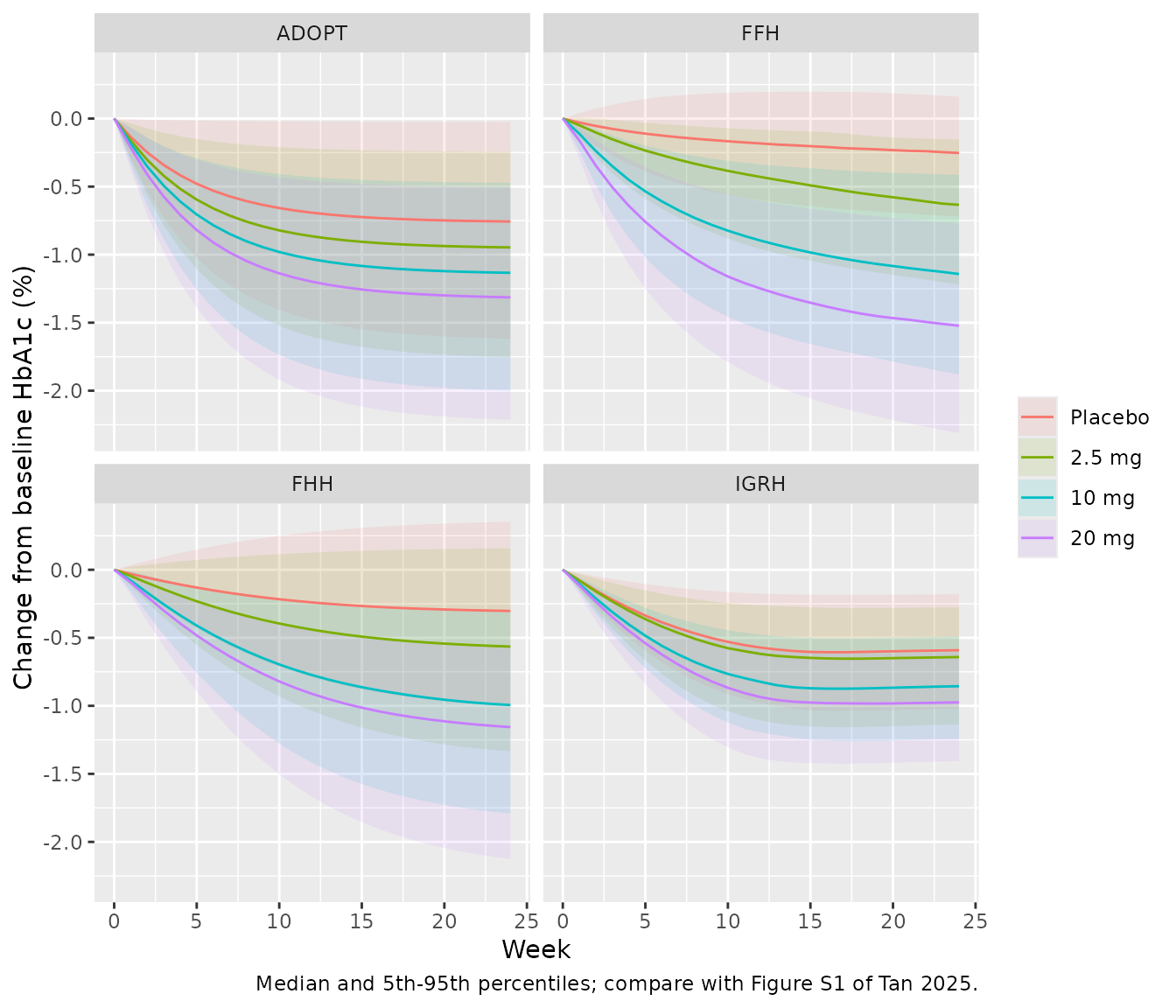
Figure S1: time course of the change in HbA1c
hba1c |>
  group_by(model, arm, time) |>
  summarise(
    Q05 = quantile(dHba1c, 0.05), Q50 = median(dHba1c), Q95 = quantile(dHba1c, 0.95),
    .groups = "drop"
  ) |>
  ggplot(aes(time / week, Q50, colour = arm, fill = arm)) +
  geom_ribbon(aes(ymin = Q05, ymax = Q95), alpha = 0.12, colour = NA) +
  geom_line() +
  facet_wrap(~model) +
  labs(
    x = "Week", y = "Change from baseline HbA1c (%)", colour = NULL, fill = NULL,
    caption = "Median and 5th-95th percentiles; compare with Figure S1 of Tan 2025."
  )
Glucose response
glu <- bind_rows(
  sims$ADOPT |> filter(time %in% pd_times) |> transmute(model = "ADOPT (AG)", id, arm, time, g = glucose),
  sims$FFH |> filter(time %in% pd_times) |> transmute(model = "FFH (FPG)", id, arm, time, g = fpg),
  sims$FHH |> filter(time %in% pd_times) |> transmute(model = "FHH (FPG)", id, arm, time, g = glucose),
  sims$IGRH |> filter(time %in% pd_times) |> transmute(model = "IGRH (AG)", id, arm, time, g = glucose)
) |>
  mutate(arm = factor(arm, levels = arm_levels))
glu |>
  group_by(model, arm, time) |>
  summarise(med = median(g), .groups = "drop") |>
  ggplot(aes(time / week, med, colour = arm)) +
  geom_line() +
  facet_wrap(~model) +
  labs(x = "Week", y = "Median glucose (mmol/L)", colour = NULL)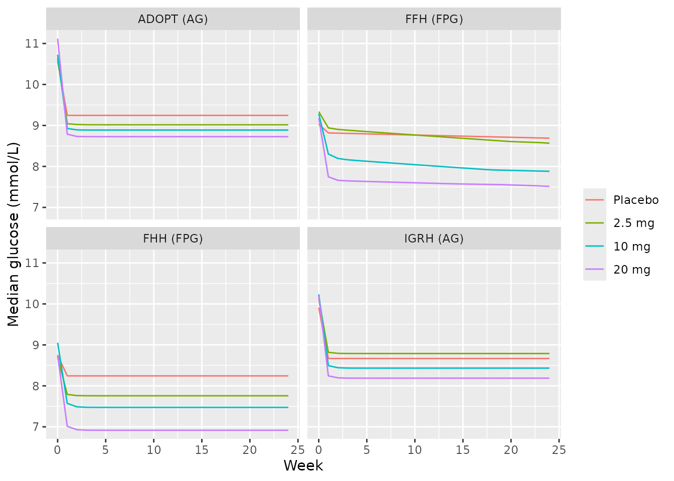
Deterministic checks
Baseline HbA1c against the closed-form steady state
For a typical patient (70 kg male, baseline FPG 8.2 mmol/L, FSI 6.86
uU/mL) each model’s HbA1c at time zero must equal the steady state of
its own structure, computed here independently of the model code. For
the transit models, with glycation rate g and transit rate
k per compartment, the non-glycated amount in compartment
j is rho^(j-1) times that in the first,
rho = k / (k + g), and total hemoglobin is the production
rate times the residence time.
typ <- tibble(id = 1L, time = c(0, 24 * week), evid = 0L, amt = 0, cmt = "central", dvid = 1L,
              WT = 70, SEXF = 0, FPG = 8.2, INS_BL = 22.5 / (0.40 * 8.2), PLACEBO = 1L)
bl_sim <- sapply(mods, function(nm) {
  s <- rxode2::rxSolve(rxode2::zeroRe(readModelDb(nm)), events = typ, useLinCmt = FALSE, returnType = "data.frame")
  s$Hba1c[1]
})
#> ℹ parameter labels from comments will be replaced by 'label()'
#> ℹ omega/sigma items treated as zero: 'etalka', 'etalcl', 'etalvc', 'etalrbase_glucose', 'etaplac'
#> ℹ parameter labels from comments will be replaced by 'label()'
#> ℹ omega/sigma items treated as zero: 'etalka', 'etalcl', 'etalvc', 'etaplac', 'etalkout_hba1c'
#> ℹ parameter labels from comments will be replaced by 'label()'
#> ℹ omega/sigma items treated as zero: 'etalka', 'etalcl', 'etalvc', 'etalrbase_glucose', 'etaplac', 'etalmtt_rbc', 'etalgamma'
#> ℹ parameter labels from comments will be replaced by 'label()'
#> ℹ omega/sigma items treated as zero: 'etalka', 'etalcl', 'etalvc', 'etalrbase_glucose', 'etaplac', 'etallsp'

transit_hba1c <- function(n, ls_day, g_day, prec = 1) {
  k <- n / ls_day
  r <- k / (k + g_day)
  non <- prec / (k + g_day) * sum(r^(0:(n - 1)))
  100 * (1 - non / ls_day)
}
ag_igrh <- 10.1 * 18.016
bl_closed <- c(
  ADOPT = 0.000706 * (9.62 + 3) / 0.00118,
  FFH = 0.000906 * 8.2 / 0.000955,
  FHH = transit_hba1c(4, 120, 0.000224 * 8.72^0.741),
  IGRH = transit_hba1c(12, 120 * (ag_igrh / 149)^-0.427, 6.76e-6 * ag_igrh, exp(-6.76e-6 * ag_igrh * 7.12))
)
knitr::kable(data.frame(model = names(mods), simulated = bl_sim, closed_form = bl_closed), digits = 5, row.names = FALSE)| model | simulated | closed_form |
|---|---|---|
| ADOPT | 7.55061 | 7.55061 |
| FFH | 7.77927 | 7.77927 |
| FHH | 7.83237 | 7.83237 |
| IGRH | 7.78147 | 7.78147 |
Steady state holds without treatment
With the placebo effect and the FFH disease progression switched off and no drug, every model must stay at its baseline for 24 weeks; any error in the 8- or 24-compartment initial conditions would show up as drift.
hold <- sapply(names(mods), function(m) {
  mod0 <- rxode2::zeroRe(readModelDb(mods[[m]]))
  mod0 <- if (m == "FFH") {
    mod0 |> rxode2::ini(plac = 0, dp_bcf = 0, dp_bcf_drug = 0, dp_is = 0)
  } else {
    mod0 |> rxode2::ini(plac = 0)
  }
  s <- rxode2::rxSolve(mod0, events = typ, useLinCmt = FALSE, returnType = "data.frame")
  abs(s$Hba1c[2] / s$Hba1c[1] - 1)
})
#> ℹ parameter labels from comments will be replaced by 'label()'
#> ℹ change initial estimate of `plac` to `0`
#> ℹ omega/sigma items treated as zero: 'etalka', 'etalcl', 'etalvc', 'etalrbase_glucose', 'etaplac'
#> ℹ parameter labels from comments will be replaced by 'label()'
#> ℹ change initial estimate of `plac` to `0`
#> ℹ change initial estimate of `dp_bcf` to `0`
#> ℹ change initial estimate of `dp_bcf_drug` to `0`
#> ℹ change initial estimate of `dp_is` to `0`
#> ℹ omega/sigma items treated as zero: 'etalka', 'etalcl', 'etalvc', 'etaplac', 'etalkout_hba1c'
#> ℹ parameter labels from comments will be replaced by 'label()'
#> ℹ change initial estimate of `plac` to `0`
#> ℹ omega/sigma items treated as zero: 'etalka', 'etalcl', 'etalvc', 'etalrbase_glucose', 'etaplac', 'etalmtt_rbc', 'etalgamma'
#> ℹ parameter labels from comments will be replaced by 'label()'
#> ℹ change initial estimate of `plac` to `0`
#> ℹ omega/sigma items treated as zero: 'etalka', 'etalcl', 'etalvc', 'etalrbase_glucose', 'etaplac', 'etallsp'
hold
#>        ADOPT          FFH          FHH         IGRH
#> 0.000000e+00 0.000000e+00 1.110223e-15 1.576517e-14
stopifnot(all(hold < 1e-6))
PKNCA validation
The paper reports no NCA, so the PK check is internal: at steady state (day 28, roughly 11 half-lives after the first dose) the AUC over a dosing interval must equal dose / CL/F for every subject.
# rxSolve's keep= drops a column named `dose`, so it is joined back by id.
pk <- sims$ADOPT |>
  left_join(cohort |> select(id, dose), by = "id") |>
  filter(dose > 0, (time >= 0 & time <= 24) | (time >= 648 & time <= 672)) |>
  filter(!is.na(Cc)) |>
  select(id, time, Cc, arm, dose, cl)
dose_rows <- pk |> distinct(id, arm, dose) |> tidyr::crossing(time = c(0, 648))

conc_obj <- PKNCA::PKNCAconc(pk, Cc ~ time | arm + id)
dose_obj <- PKNCA::PKNCAdose(dose_rows, dose ~ time | arm + id)
intervals <- data.frame(
  start = c(0, 648), end = c(24, 672),
  cmax = TRUE, tmax = TRUE, auclast = TRUE, cav = TRUE
)
nca <- PKNCA::pk.nca(PKNCA::PKNCAdata(conc_obj, dose_obj, intervals = intervals))
summary(nca)
#>  start end    arm   N      auclast        cmax              tmax         cav
#>      0  24  10 mg 150  6110 [22.5]  290 [22.3] 9.00 [5.50, 14.5]  255 [22.5]
#>    648 672  10 mg 150 27600 [26.3] 1240 [25.9] 5.50 [4.00, 7.50] 1150 [26.3]
#>      0  24 2.5 mg 150  1490 [23.8] 70.7 [23.5] 9.50 [6.00, 14.0] 61.9 [23.8]
#>    648 672 2.5 mg 150  6660 [29.1]  299 [28.6] 5.50 [4.00, 7.50]  278 [29.1]
#>      0  24  20 mg 150 11800 [25.4]  564 [25.2] 9.50 [6.00, 15.0]  493 [25.4]
#>    648 672  20 mg 150 52400 [31.6] 2350 [30.9] 5.50 [4.00, 7.50] 2180 [31.6]
#>
#> Caption: auclast, cmax, cav: geometric mean and geometric coefficient of variation; tmax: median and range; N: number of subjects
ss <- as.data.frame(nca$result) |>
  filter(PPTESTCD == "auclast", start == 648) |>
  left_join(pk |> distinct(id, dose, cl), by = "id") |>
  mutate(ratio = PPORRES / (1000 * dose / cl))
summary(ss$ratio)
#>    Min. 1st Qu.  Median    Mean 3rd Qu.    Max.
#>  0.9967  0.9993  0.9995  0.9994  0.9997  0.9999
stopifnot(
  nrow(ss) == 3 * n_arm,
  # Same drawn CL on both sides: only trapezoidal error on a 0.5-h grid remains.
  abs(median(ss$ratio) - 1) < 0.01,
  all(abs(ss$ratio - 1) < 0.03)
)
Assumptions and deviations
- Equations from the original frameworks. Tan 2025 gives no equations; it names the four frameworks, shows their compartment diagrams (Figure 2) and reports the final estimates (Tables S2-S6). The ODEs, initial conditions, HOMA constants (5 and 22.5, with 3.5 mmol/L as the glucose threshold) and the 149 mg/dL reference glucose of the IGRH lifespan come from the NONMEM implementations deposited by Kunina 2022 (supplements S2-S6), which share authors with the Lilly team behind Tan 2025.
-
How placebo and drug combine is not stated. Both
reduce the glucose input and are applied multiplicatively,
(1 - PLAC) * (1 - IMAX * C / (IC50 + C)). The maintainers compared this with an additive form1 - PLAC - Imax(C)against Table 2: the multiplicative form reproduced the ADOPT predictions much more closely (root-mean-square difference over the four arms 0.025% vs 0.074%) and the IGRH predictions somewhat more closely (0.028% vs 0.040%), the two forms were equivalent for FFH, and the additive form was slightly closer for FHH (0.033% vs 0.047%). One form is used for all four models since they share the authors’ code base. Placebo starts at time zero for every patient. -
IGRH precursor glycation is dynamic, i.e. the
fraction of hemoglobin glycated during the precursor lifespan,
exp(-KGL * AG * LSP), follows the current AG, as in the original Lledo-Garcia 2013 model and the Bosch 2025 implementation in this package (Bosch_2025_glp1ra_hba1c). Freezing it at baseline, as in the Kunina 2022 code, under-predicts the Table 2 IGRH column by 0.09-0.20%. - IGRH lifespan exponent sign. Table S6 reports GAMMA = 0.427 for the AG effect on RBC lifespan, which “decreased less than proportionally with higher AG”; it is coded as the exponent -0.427 of (AG / 149 mg/dL), so the lifespan is 120 days at 149 mg/dL. AG is converted from mmol/L with 18.016 mg/dL per mmol/L.
-
FFH baselines are covariates. Table S4 has no
baseline glucose or insulin parameter, consistent with the text:
baseline beta-cell function and insulin sensitivity are derived from
each patient’s observed baseline FPG (
FPG) and fasting insulin (INS_BL, uU/mL) by HOMA. The disease-progression coefficients are added on the logit scale per year, the form in which a positive coefficient is the deterioration the Table S4 footnote describes and 0.1/year moves a 40% insulin sensitivity by about 2% per year, as the Results state. The additional beta-cell term applies to drug-treated patients (PLACEBO = 0). The placebo effect is switched on fort > 0, so the algebraic FPG and FSI equal their observed baselines at time zero. - Fasting serum glucose was used by the authors in place of fasting plasma glucose; the models’ fasting glucose output is that measurement.
-
Hemoglobin. In FHH total hemoglobin (g/L) is an
observed output. In IGRH it is computed (
hb) but was not fitted; KINHB was fixed to the value whose simulated baseline Hb best matched the observed baselines. - Residual errors are the proportional SDs of Tables S2-S6.
- Virtual cohort. Covariates are drawn from the Phase 2b means and SDs of Table 1 rather than resampled from the individual data; baseline insulin is assumed (see above), and 150 patients per arm are simulated instead of 200 studies of 65 per arm, so the comparison is against the published mean predictions only.
- Not reproduced. The bias and precision metrics (Figure 4, Table 3) and the observed-versus-predicted intervals (Figure 3) need the individual Phase 2b observations.