Dapagliflozin (Kobuchi 2025)
Source:vignettes/articles/Kobuchi_2025_dapagliflozin.Rmd
Kobuchi_2025_dapagliflozin.RmdModel and source
Citation: Kobuchi S, Sakai S, Terada R, Kato KI, Hayakawa T, Sakaeda T. Population Pharmacokinetic-pharmacodynamic Model Analysis of Dapagliflozin for HbA1c-lowering Effects in Japanese Patients with Type 2 Diabetes Mellitus using Long-term Real-world Data. Int J Med Sci. 2025;22(10):2333-2341. doi:10.7150/ijms.111519. The HbA1c turnover-with-Emax structure is inherited from de Winter W, Dunne A, de Trixhe XW, et al. Br J Clin Pharmacol. 2017;83(5):1072-1081 (canagliflozin). ka and V/F were fixed from Melin J, Parkinson J, Hamren B, et al. Br J Clin Pharmacol. 2024;90(2):606-612.
Description: One-compartment first-order-absorption population PK model for oral dapagliflozin coupled to a turnover (indirect-response) Emax model for the HbA1c-lowering effect, in Japanese outpatients with type 2 diabetes mellitus treated with 5 mg once daily for one year in routine clinical practice (long-term real-world data). Absorption rate constant and apparent volume of distribution were FIXED from a prior dapagliflozin population PK analysis (Melin 2024) because all study samples were trough concentrations; apparent clearance was estimated with a power effect of time-varying body weight. HbA1c is described by a zero-order production / first-order loss turnover pool whose loss rate is parameterised by the HbA1c half-life; drug effect is a fractional Emax inhibition of production scaled by the subject’s own baseline HbA1c relative to a reference baseline of 8.0% above a 5.0% normoglycemia floor. Two endpoints are declared: plasma dapagliflozin concentration (Cc, ng/mL) and HbA1c (%).
Article: https://doi.org/10.7150/ijms.111519
Supplement (goodness-of-fit plots, covariate-selection table): https://www.medsci.org/v22p2333s1.pdf
Kobuchi 2025 links a one-compartment first-order-absorption population PK model for oral dapagliflozin to a turnover (indirect-response) model with an Emax drug effect on HbA1c production. The PD structure is inherited from de Winter 2017 (canagliflozin). The distinguishing feature of this paper is that both layers were fit to long-term real-world data – one year of routine-care observations rather than a controlled trial.
Population
| Field | Value |
|---|---|
| Species | human |
| N subjects | 85 |
| Studies | 1 |
| Age | 59 years (37-75 years) |
| Weight | 77.0 kg (49.0-118.0 kg) |
| Female | 28.2% |
| Region | Japan (single centre, Tonami General Hospital, Toyama) |
| Observations | 415 plasma dapagliflozin concentrations (all trough) and 508 HbA1c values |
Eighty-five Japanese outpatients with type 2 diabetes mellitus, treated at a single centre (Tonami General Hospital, Toyama) with dapagliflozin 5 mg once daily after breakfast for 12 months. All patients were already on metformin (1000 mg/day or more) plus a DPP-4 inhibitor before dapagliflozin was started. Baseline HbA1c was 6.8% (SD 0.5, range 5.6-8.8), body weight 77.0 kg (range 49.0-118.0), eGFR 74.3 mL/min/1.73 m2 (range 39.2-137.8). Visits occurred at 1, 3, 6, 9 and 12 months with overnight fasting, yielding 415 plasma dapagliflozin concentrations – all of them troughs – and 508 HbA1c values.
Because every PK sample was a trough, ka and
V/F are not identifiable from this dataset and were fixed
from a prior dapagliflozin population PK analysis (Melin 2024). The
PK-PD model was fit sequentially: individual post hoc
PK parameters from the PK model were held fixed while the HbA1c
parameters were estimated.
The same information is available programmatically via
readModelDb("Kobuchi_2025_dapagliflozin")()$population.
Source trace
The per-parameter origin is recorded as an in-file comment next to
each ini() entry in
inst/modeldb/specificDrugs/Kobuchi_2025_dapagliflozin.R.
The table below collects them in one place for review.
| Equation / parameter | Value | Source location |
|---|---|---|
lka (ka) |
57.4 1/day, FIXED | Table 2, row “k a (1/day)”; CV% column reads “Fix” |
lcl (CL/F) |
229.3 L/day | Table 2, row “theta CL/F”; Results text “population mean CL/F was 229.3 L/day (1.5% CV)” |
e_wt_cl |
0.41 | Table 2, row “theta BW”; Results text “0.41 (2.5%-97.5%CI: 0.24-0.58) is the exponential coefficient of body weight” |
lvc (V/F) |
73.9 L, FIXED | Table 2, row “V/F (L)”; CV% column reads “Fix” |
lthalfrec (t1/2HbA1c) |
16.1 day | Table 3, row “t 1/2 HbA1c (day)” |
lemax (Emax) |
0.034 HbA1c %/day | Table 3, row “E max (HbA1c %/day)” |
lec50 (EC50) |
23.7 ng/mL | Table 3, row “EC 50 (ng/mL)” |
etalcl |
omega = 13.9% -> var 0.019321 | Table 2, row “omega CL/F (%)” |
etalthalfrec |
omega = 103.9% -> var 1.079521 | Table 3, row “omega t1/2 HbA1c (%)” |
propSd |
39.8% | Table 2, row “sigma (%)”; Results “multiplicative error correction” |
addSd_hba1c |
0.24 HbA1c % | Table 3, row “sigma (HbA1c %)”; Results “additive error correction” |
| CL/F covariate model | CL/F = theta_CL/F * (BW/77.0)^theta_BW |
Table 2 row header; unnumbered equation in Results “Population PK model” |
d/dt(hba1c) |
n/a | Equation 2, page 2335 |
ef (baseline scaling) |
n/a | Equation 3, page 2335 |
efc (Emax term) |
n/a | Equation 4, page 2335 |
kout |
n/a | Equation 5, page 2335 |
kin = HBA1C * kout |
n/a | Derived from equation 2 at dH(0) = 0; see Errata |
| 5.0% floor, 8.0% reference | n/a | Equation 3 and Table 3 footnote |
Virtual cohort
Original observed data are not publicly available. The cohort below approximates the published baseline demographics: body weight from a normal distribution (mean 78.1, SD 13.4) truncated to the observed 49-118 kg range, and baseline HbA1c from a normal distribution (mean 6.8, SD 0.5) truncated to the observed 5.6-8.8% range (Kobuchi 2025 Table 1).
Two arms are simulated – the studied 5 mg/day regimen and the 10 mg/day regimen that Kobuchi 2025 Figure 4 extrapolates – at 200 subjects per arm.
set.seed(20250422)
n_per_arm <- 200L

rtnorm <- function(n, mean, sd, lo, hi) {
  x <- rnorm(n, mean, sd)
  while (any(bad <- x < lo | x > hi)) x[bad] <- rnorm(sum(bad), mean, sd)
  x
}

# Steady-state sampling window: the final dosing interval (day 364 -> 365).
ss_start <- 364
ss_end   <- 365

# Trough grid across the treatment year (all published PK samples were troughs)
# plus a dense profile through the final dosing interval so Tmax is resolved
# and AUC0-tau is not discretisation-biased.
obs_times <- sort(unique(c(
  seq(0, 364, by = 7),
  ss_start + c(seq(0, 0.2, by = 0.005), seq(0.25, 1, by = 0.025))
)))

make_arm <- function(n, dose_mg, label, id_offset = 0L) {
  subj <- tibble(
    id        = id_offset + seq_len(n),
    WT        = rtnorm(n, 78.1, 13.4, 49, 118),
    HBA1C     = rtnorm(n, 6.8, 0.5, 5.6, 8.8),
    treatment = label
  )
  doses <- subj |>
    mutate(time = 0, amt = dose_mg, evid = 1L, cmt = "depot",
           ii = 1, addl = 364)
  obs <- subj |>
    tidyr::crossing(time = obs_times) |>
    mutate(amt = NA_real_, evid = 0L,
           # `cmt = "Cc"` is REQUIRED here: this model declares two endpoints
           # (Cc and hba1c), so rxode2 maps observation rows onto endpoint
           # slots. `cmt = "central"` fails with "undefined compartment".
           # lint_vignette.R flags this as [cmt-observable]; that warning is a
           # false positive for declared multi-endpoint models.
           cmt = "Cc", ii = 0, addl = 0L)
  bind_rows(doses, obs) |>
    # Observations sort BEFORE the same-time dose so day-7k samples are
    # pre-dose troughs, matching the paper's sampling.
    arrange(id, time, evid)
}

events <- bind_rows(
  make_arm(n_per_arm,  5, "5 mg/day",  id_offset = 0L),
  make_arm(n_per_arm, 10, "10 mg/day", id_offset = n_per_arm)
)
stopifnot(!anyDuplicated(unique(events[, c("id", "time", "evid")])))
stopifnot(dplyr::n_distinct(events$id) == 2L * n_per_arm)
Simulation
# `readModelDb()` returns the model FUNCTION; resolve it to an rxUi once so
# `$omega` and the other accessors work (`ui` was built in the metadata chunk).
mod <- ui

sim <- rxode2::rxSolve(
  mod, events = events,
  omega     = mod$omega,   # pass omega explicitly; rxSolve reuses a stale one otherwise
  useLinCmt = FALSE,       # ODE -> linCmt auto-conversion corrupts the dvid mapping
  keep      = c("treatment", "WT", "HBA1C"),
  returnType = "data.frame"
)

# rxSolve silently drops subjects on failure -- assert the count survived.
stopifnot(dplyr::n_distinct(sim$id) == 2L * n_per_arm)
# Assert IIV was actually applied (a stale omega would collapse all subjects).
stopifnot(dplyr::n_distinct(round(sim$cl, 8)) > 1L)
Cc is the individual prediction without residual error;
the sim column carries the residual error. Figures and NCA
below use Cc, which is the quantity the paper’s structural
equations define.
Replicate published figures
Figure 2 – plasma dapagliflozin concentrations over 12 months
Kobuchi 2025 Figure 2 is a prediction-corrected VPC of trough dapagliflozin concentrations. The panel below shows the simulated trough profile for the studied 5 mg/day regimen.
# Replicates Figure 2 of Kobuchi 2025: trough dapagliflozin concentration
# over the 12-month treatment period.
sim |>
  filter(treatment == "5 mg/day", time %in% seq(0, 364, by = 7), time > 0) |>
  group_by(time) |>
  summarise(Q05 = quantile(Cc, 0.05), Q50 = median(Cc),
            Q95 = quantile(Cc, 0.95), .groups = "drop") |>
  ggplot(aes(time, Q50)) +
  geom_ribbon(aes(ymin = Q05, ymax = Q95), alpha = 0.25, fill = "steelblue") +
  geom_line(linewidth = 0.8, colour = "steelblue4") +
  labs(x = "Time (day)", y = "Trough dapagliflozin (ng/mL)",
       title = "Figure 2 -- simulated trough concentrations, 5 mg/day",
       caption = "Replicates Figure 2 of Kobuchi 2025 (median with 5th-95th percentiles).")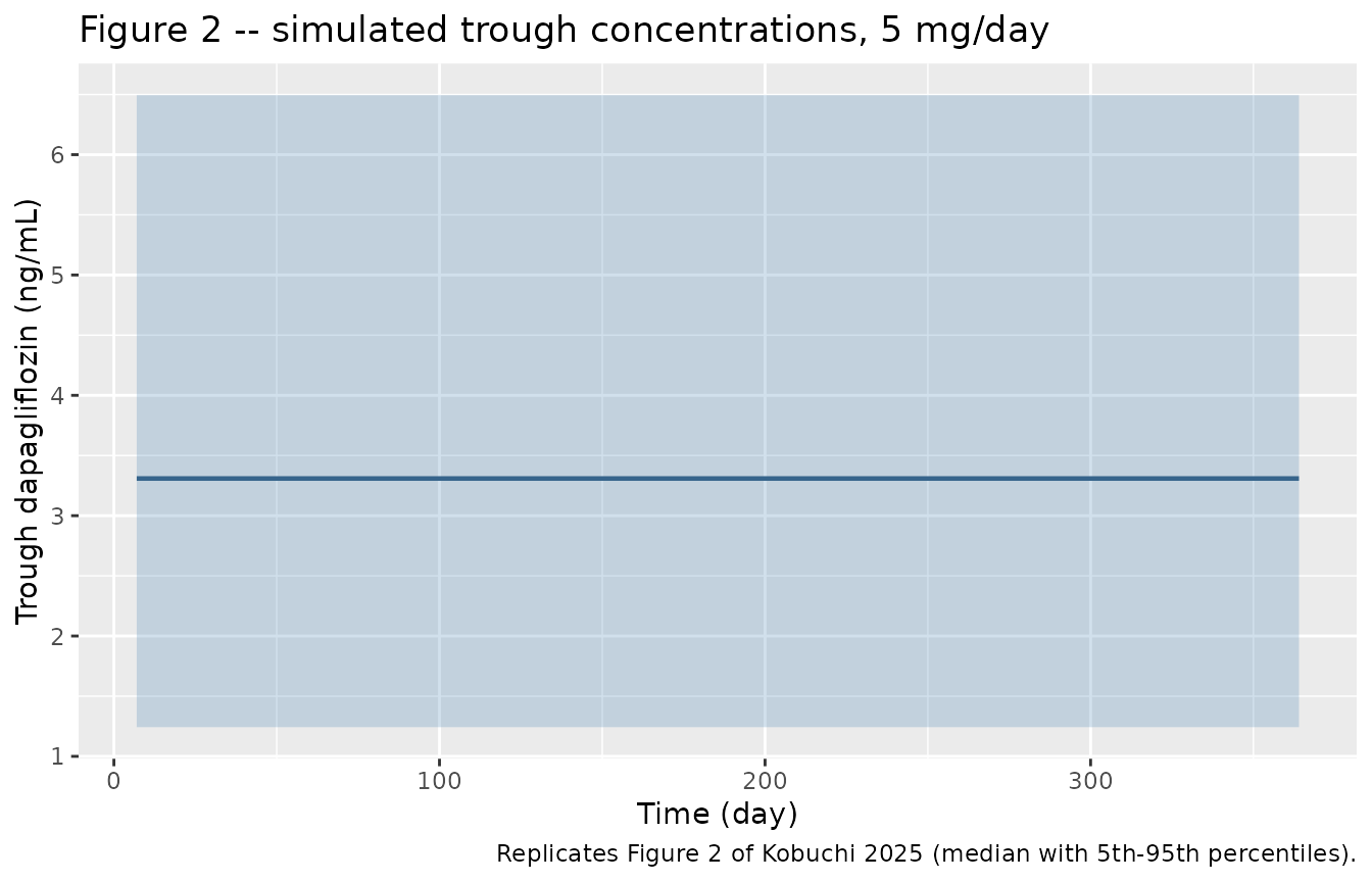
Figure 3 – HbA1c over 12 months
# Replicates Figure 3 of Kobuchi 2025: HbA1c time profile, 5 mg/day.
sim |>
  filter(treatment == "5 mg/day", time %in% seq(0, 364, by = 7)) |>
  group_by(time) |>
  summarise(Q05 = quantile(hba1c, 0.05), Q50 = median(hba1c),
            Q95 = quantile(hba1c, 0.95), .groups = "drop") |>
  ggplot(aes(time, Q50)) +
  geom_ribbon(aes(ymin = Q05, ymax = Q95), alpha = 0.25, fill = "firebrick") +
  geom_line(linewidth = 0.8, colour = "firebrick4") +
  labs(x = "Time (day)", y = "HbA1c (%)",
       title = "Figure 3 -- simulated HbA1c, 5 mg/day",
       caption = "Replicates Figure 3 of Kobuchi 2025 (median with 5th-95th percentiles).")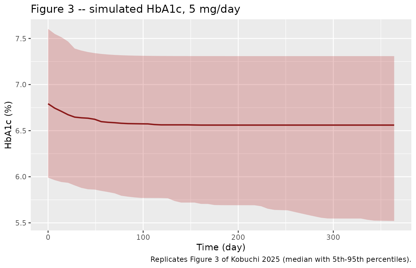
Figure 4 – 5 mg versus 10 mg once daily
# Replicates Figure 4 of Kobuchi 2025: simulated HbA1c for 5 vs 10 mg/day.
sim |>
  filter(time %in% seq(0, 364, by = 7)) |>
  group_by(time, treatment) |>
  summarise(Q05 = quantile(hba1c, 0.05), Q50 = median(hba1c),
            Q95 = quantile(hba1c, 0.95), .groups = "drop") |>
  ggplot(aes(time, Q50, colour = treatment, fill = treatment)) +
  geom_ribbon(aes(ymin = Q05, ymax = Q95), alpha = 0.18, colour = NA) +
  geom_line(linewidth = 0.8) +
  labs(x = "Time (day)", y = "HbA1c (%)", colour = NULL, fill = NULL,
       title = "Figure 4 -- HbA1c after 5 or 10 mg/day dapagliflozin",
       caption = "Replicates Figure 4 of Kobuchi 2025 (median with 5th-95th percentiles).")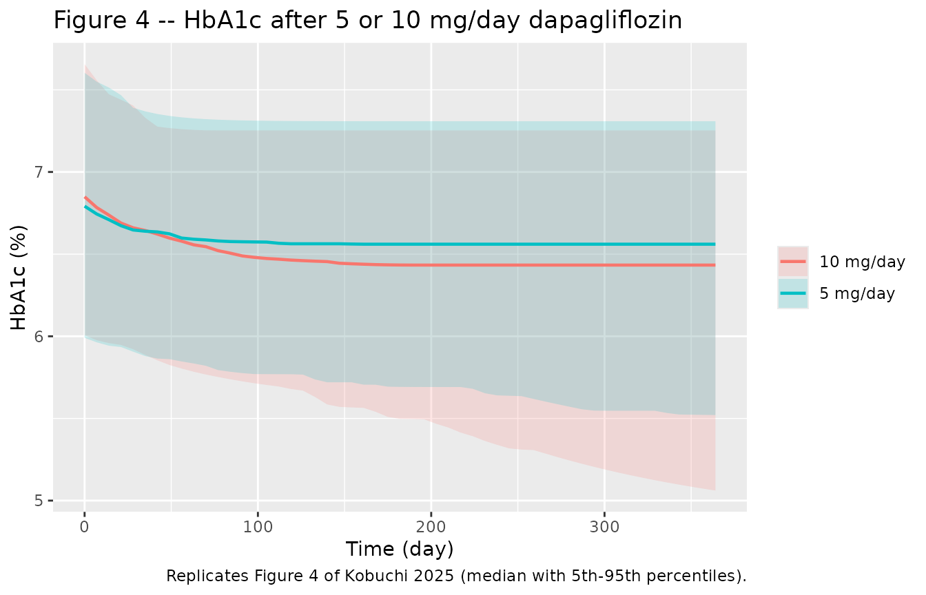
Kobuchi 2025 reports the simulated HbA1c at 12 months as a median with a 5th to 95th percentile range. The table below compares those published values against the packaged model.
hba1c_12mo <- sim |>
  filter(time == 364) |>
  group_by(treatment) |>
  summarise(sim_med = median(hba1c), sim_p05 = quantile(hba1c, 0.05),
            sim_p95 = quantile(hba1c, 0.95), .groups = "drop")

published_hba1c <- tibble::tribble(
  ~treatment,   ~pub_med, ~pub_p05, ~pub_p95,
  "5 mg/day",   6.5,      5.6,      7.4,
  "10 mg/day",  6.4,      5.4,      7.4
)

baseline_row <- sim |>
  filter(time == 0) |>
  summarise(treatment = "Baseline (both arms)",
            sim_med = median(hba1c), sim_p05 = quantile(hba1c, 0.05),
            sim_p95 = quantile(hba1c, 0.95)) |>
  mutate(pub_med = 6.8, pub_p05 = 6.0, pub_p95 = 7.8)

hba1c_12mo |>
  left_join(published_hba1c, by = "treatment") |>
  bind_rows(baseline_row) |>
  mutate(across(where(is.numeric), \(x) round(x, 2))) |>
  transmute(
    "HbA1c (%)"          = treatment,
    "Simulated median"   = sim_med,
    "Published median"   = pub_med,
    "Simulated 5th-95th" = paste0(sim_p05, " - ", sim_p95),
    "Published 5th-95th" = paste0(pub_p05, " - ", pub_p95)
  ) |>
  knitr::kable(caption = paste(
    "HbA1c at 12 months, simulated vs Kobuchi 2025 Figure 4 / Simulation text.",
    "Baseline row is the virtual cohort's own starting distribution."
))| HbA1c (%) | Simulated median | Published median | Simulated 5th-95th | Published 5th-95th |
|---|---|---|---|---|
| 10 mg/day | 6.43 | 6.4 | 5.06 - 7.25 | 5.4 - 7.4 |
| 5 mg/day | 6.56 | 6.5 | 5.52 - 7.31 | 5.6 - 7.4 |
| Baseline (both arms) | 6.83 | 6.8 | 5.99 - 7.66 | 6 - 7.8 |
The simulated medians reproduce the published 6.5% (5 mg) and 6.4% (10 mg) to the reported precision. The percentile bands are close but not exact, and the deviation runs in both directions: the 95th percentile is ~0.1-0.15% low in both arms, and the 5th percentile is ~0.1% low at 5 mg and ~0.3% low at 10 mg.
Both tails trace to the same cause – the virtual cohort’s baseline
HbA1c is a symmetric truncated normal, whereas the
observed baseline distribution is right-skewed (the published simulated
baseline band is 6.0-7.8% around a median of 6.8%, i.e. -0.8/+1.0). The
cohort chunk reproduces the baseline median and the lower tail but falls
~0.15% short at the top, and because the HbA1c deficit is exactly
proportional to H(0) - 5 that shortfall propagates to the
12-month upper percentile. The wider lower tail at 10 mg is the large
IIV on t1/2HbA1c (omega = 103.9%) acting on the larger 10
mg effect: subjects drawn with a long HbA1c half-life get a
proportionally larger deficit. Individual baseline HbA1c values are not
published, so the skew cannot be reproduced exactly without the source
data.
PKNCA validation
NCA is run on the final dosing interval (day 364 to 365), i.e. at steady state.
sim_nca <- sim |>
  filter(!is.na(Cc), time >= ss_start, time <= ss_end) |>
  select(id, time, Cc, treatment)

stopifnot(nrow(sim_nca) > 0)
stopifnot(all(sim_nca$Cc >= 0))

conc_obj <- PKNCA::PKNCAconc(as.data.frame(sim_nca), Cc ~ time | treatment + id)

dose_df <- events |>
  filter(evid == 1) |>
  distinct(id, treatment) |>
  mutate(time = ss_start,
         amt = if_else(treatment == "5 mg/day", 5, 10))

dose_obj <- PKNCA::PKNCAdose(as.data.frame(dose_df), amt ~ time | treatment + id)

intervals <- data.frame(
  start   = ss_start,
  end     = ss_end,
  cmax    = TRUE,
  tmax    = TRUE,
  cmin    = TRUE,
  auclast = TRUE,
  cav     = TRUE
)

nca_res <- PKNCA::pk.nca(PKNCA::PKNCAdata(conc_obj, dose_obj, intervals = intervals))
Structural identity: AUC0-tau equals Dose / (CL/F)
At steady state with once-daily dosing, AUC0-tau must
equal Dose / (CL/F) for every subject. This is a
per-subject identity, not a median comparison, so it is a strict check
on the packaged PK parameterisation and on the unit conversion between
mg/L and ng/mL.
auc_tau <- as.data.frame(nca_res) |>
  filter(PPTESTCD == "auclast") |>
  select(id, treatment, auc_nca = PPORRES)

cl_by_id <- sim |>
  distinct(id, treatment, cl) |>
  mutate(dose_mg = if_else(treatment == "5 mg/day", 5, 10),
         # Dose (mg) / CL (L/day) = mg/L over one day; x 1000 -> ng*day/mL
         auc_theory = dose_mg / cl * 1000)

auc_check <- auc_tau |>
  inner_join(cl_by_id, by = c("id", "treatment")) |>
  mutate(pct_diff = 100 * (auc_nca - auc_theory) / auc_theory)

stopifnot(nrow(auc_check) == 2L * n_per_arm)
# Residual gap is pure trapezoidal discretisation of a sharp absorption peak.
# Observed max is ~0.06%; the bound is set just above that so the check stays
# sensitive to a real regression rather than merely "not obviously broken".
stopifnot(max(abs(auc_check$pct_diff)) < 0.2)

auc_check |>
  group_by(treatment) |>
  summarise(
    n = n(),
    `Median AUC0-tau, NCA (ng*day/mL)`      = round(median(auc_nca), 3),
    `Median Dose/(CL/F) (ng*day/mL)`        = round(median(auc_theory), 3),
    `Max |difference| (%)`                  = round(max(abs(pct_diff)), 3),
    .groups = "drop"
  ) |>
  rename("Treatment" = treatment, "N" = n) |>
knitr::kable(caption = "Per-subject steady-state AUC0-tau against the closed-form Dose/(CL/F).")| Treatment | N | Median AUC0-tau, NCA (ng*day/mL) | Median Dose/(CL/F) (ng*day/mL) | Max |difference| (%) |
|---|---|---|---|---|
| 10 mg/day | 200 | 44.404 | 44.421 | 0.060 |
| 5 mg/day | 200 | 21.684 | 21.693 | 0.057 |
Comparison against published exposure
Kobuchi 2025 reports no NCA table. The one directly comparable
published exposure statement is the trough level: the Introduction cites
average trough concentrations of 2-5 ng/mL in this
cohort on 5 mg/day (from the same authors’ earlier report on 72 of these
patients). PKNCA’s ctrough is known to return
NA on steady-state intervals, so the end-of-interval
concentration is read directly off the solved profile; for this
monotonically declining plasma profile it coincides with
cmin.
trough <- sim |>
  filter(time == ss_end) |>
  group_by(treatment) |>
  summarise(med = median(Cc), p05 = quantile(Cc, 0.05),
            p95 = quantile(Cc, 0.95), .groups = "drop")

cmin_pknca <- as.data.frame(nca_res) |>
  filter(PPTESTCD == "cmin") |>
  group_by(treatment) |>
  summarise(cmin_med = median(PPORRES), .groups = "drop")

trough |>
  left_join(cmin_pknca, by = "treatment") |>
  mutate(across(where(is.numeric), \(x) round(x, 2)),
         published = if_else(treatment == "5 mg/day",
                             "2 - 5 (average trough, Kobuchi 2025 Introduction)",
                             "not reported (10 mg not administered in this cohort)")) |>
  transmute(
    "Treatment"                        = treatment,
    "Simulated trough, median (ng/mL)" = med,
    "Simulated trough, 5th-95th"       = paste0(p05, " - ", p95),
    "PKNCA cmin, median (ng/mL)"       = cmin_med,
    "Published (ng/mL)"                = published
  ) |>
knitr::kable(caption = "Steady-state trough dapagliflozin concentration vs the published range.")| Treatment | Simulated trough, median (ng/mL) | Simulated trough, 5th-95th | PKNCA cmin, median (ng/mL) | Published (ng/mL) |
|---|---|---|---|---|
| 10 mg/day | 7.13 | 2.76 - 15.43 | 7.13 | not reported (10 mg not administered in this cohort) |
| 5 mg/day | 3.31 | 1.24 - 6.49 | 3.31 | 2 - 5 (average trough, Kobuchi 2025 Introduction) |
The simulated 5 mg/day median trough falls inside the published 2-5
ng/mL window, and the directly-read trough agrees with PKNCA’s
cmin, confirming the profile declines monotonically to the
end of the interval.
summary(nca_res)
#>  start end treatment   N     auclast        cmax        cmin
#>    364 365 10 mg/day 200 44.1 [16.6]  121 [4.62] 6.75 [56.7]
#>    364 365  5 mg/day 200 21.5 [15.4] 60.0 [4.20] 3.11 [53.6]
#>                     tmax         cav
#>  0.0550 [0.0450, 0.0600] 44.1 [16.6]
#>  0.0550 [0.0500, 0.0600] 21.5 [15.4]
#>
#> Caption: auclast, cmax, cmin, cav: geometric mean and geometric coefficient of variation; tmax: median and range; N: number of subjects
Turnover-model checks
PKNCA validates the PK layer. The HbA1c layer is a turnover model, so it is checked with the steady-state / perturbation patterns appropriate to indirect response models.
Steady-state hold: without drug, HbA1c stays at baseline
The paper assumes dH(0) = 0, which fixes
kin = kout * H(0). If that identity is encoded correctly, a
subject given no drug must hold HbA1c exactly at baseline for the whole
year, for any baseline and any t1/2HbA1c.
hold_subj <- tibble(id = 1:5, WT = c(50, 65, 77, 95, 118),
                    HBA1C = c(5.6, 6.2, 6.8, 7.5, 8.8))
hold_ev <- hold_subj |>
  tidyr::crossing(time = seq(0, 365, by = 7)) |>
  mutate(amt = NA_real_, evid = 0L, cmt = "Cc")

hold <- rxode2::rxSolve(mod, as.data.frame(hold_ev), omega = NA,
                        useLinCmt = FALSE, keep = "HBA1C",
                        returnType = "data.frame")
#> Warning: multi-subject simulation without without 'omega'

stopifnot(nrow(hold) > 0)
max_drift <- max(abs(hold$hba1c - hold$HBA1C))
stopifnot(max_drift < 1e-8)
cat(sprintf("Max |HbA1c(t) - baseline| over 1 year with no drug: %.3e %%\n", max_drift))
#> Max |HbA1c(t) - baseline| over 1 year with no drug: 0.000e+00 %
Baseline scaling of the drug effect (equation 3)
Equation 3 scales the drug effect by
(H(0) - 5) / (8 - 5). Writing the HbA1c deficit as
D = H(0) - H(t), equation 2 becomes
dD/dt = Ef - kout * D with D(0) = 0. Because
Efc depends only on the PK (identical across subjects who
share covariates) and Ef = Efc * (H(0) - 5) / 3, the
deficit D(t) is exactly proportional to
H(0) - 5 at every time point. That gives two
falsifiable identities, checked below on three baselines with otherwise
identical covariates:
- a subject sitting exactly on the 5.0% floor shows no drug effect at all;
- the ratio of deficits for baselines 8.0% and 6.5% is exactly
(8 - 5) / (6.5 - 5) = 2.
floor_subj <- tibble(id = 1:3, WT = 77, HBA1C = c(5.0, 6.5, 8.0))
floor_ev <- bind_rows(
  floor_subj |> mutate(time = 0, amt = 5, evid = 1L, cmt = "depot", ii = 1, addl = 364),
  floor_subj |> tidyr::crossing(time = seq(0, 365, by = 7)) |>
    mutate(amt = NA_real_, evid = 0L, cmt = "Cc", ii = 0, addl = 0L)
) |>
  arrange(id, time, evid)

floor_sim <- rxode2::rxSolve(mod, as.data.frame(floor_ev), omega = NA,
                             useLinCmt = FALSE, keep = "HBA1C",
                             returnType = "data.frame")
#> Warning: multi-subject simulation without without 'omega'

floor_end <- floor_sim |>
  filter(time == 364) |>
  mutate(deficit = HBA1C - hba1c)
stopifnot(nrow(floor_end) == 3L)

get_deficit <- function(baseline) {
  v <- floor_end$deficit[floor_end$HBA1C == baseline]
  if (length(v) != 1L) stop("no unique row for baseline ", baseline)
  v
}

# (1) Exactly zero effect at the 5.0% floor.
stopifnot(abs(get_deficit(5.0)) < 1e-10)
# (2) Deficit ratio is exactly (8-5)/(6.5-5) = 2.
stopifnot(abs(get_deficit(8.0) / get_deficit(6.5) - 2) < 1e-8)

floor_end |>
  transmute("Baseline HbA1c (%)"     = HBA1C,
            "HbA1c at 12 months (%)" = round(hba1c, 4),
            "Deficit H(0)-H(t) (%)"  = round(deficit, 6),
            # Undefined (0/0) on the floor row itself, so shown as NA there.
            "Deficit / (H(0)-5)"     = if_else(HBA1C > 5,
                                               round(deficit / (HBA1C - 5), 6),
                                               NA_real_)) |>
  knitr::kable(caption = paste(
    "Equation 3 baseline scaling. The last column is constant by construction:",
    "the HbA1c deficit is exactly proportional to H(0) - 5."
))| Baseline HbA1c (%) | HbA1c at 12 months (%) | Deficit H(0)-H(t) (%) | Deficit / (H(0)-5) |
|---|---|---|---|
| 5.0 | 5.0000 | 0.000000 | NA |
| 6.5 | 6.3387 | 0.161308 | 0.107539 |
| 8.0 | 7.6774 | 0.322616 | 0.107539 |
Steady-state offset matches the closed form
At steady state under a constant average effect, equation 2 gives
H_ss = H(0) - Ef / kout. Comparing the simulated 12-month
HbA1c against that closed form confirms the turnover algebra
(kin, kout, and the equation-3 scaling) is
wired together correctly.
offset_chk <- sim |>
  filter(treatment == "5 mg/day", time == 364) |>
  transmute(id, HBA1C, hba1c,
            # Effect averaged over the final dosing interval, per subject.
            drop_sim = HBA1C - hba1c)

ef_avg <- sim |>
  filter(treatment == "5 mg/day", time >= ss_start, time <= ss_end) |>
  group_by(id) |>
  # Time-average of ef over the interval by the trapezoidal rule.
  summarise(ef_bar = sum(diff(time) * (head(ef, -1) + tail(ef, -1)) / 2) /
              (max(time) - min(time)),
            kout = first(kout), .groups = "drop")

offset_chk <- offset_chk |>
  inner_join(ef_avg, by = "id") |>
  mutate(drop_theory = ef_bar / kout,
         pct_diff = 100 * (drop_sim - drop_theory) / drop_theory)

stopifnot(nrow(offset_chk) == n_per_arm)
# Subjects with a very long t1/2HbA1c are not fully at steady state by day 364,
# so the identity is asserted on the median rather than every subject. The
# observed median gap is ~0.9%; the bound is set just above it.
stopifnot(abs(median(offset_chk$pct_diff)) < 2)

tibble(
  "Quantity" = c("Median simulated HbA1c drop (%)",
                 "Median closed-form Ef / kout (%)",
                 "Median difference (%)"),
  "Value" = round(c(median(offset_chk$drop_sim), median(offset_chk$drop_theory),
                    median(offset_chk$pct_diff)), 3)
) |>
knitr::kable(caption = "Turnover steady-state offset vs the closed form H(0) - Ef/kout, 5 mg/day.")| Quantity | Value |
|---|---|
| Median simulated HbA1c drop (%) | 0.160 |
| Median closed-form Ef / kout (%) | 0.161 |
| Median difference (%) | -0.908 |
Assumptions and deviations
kinprose typo (erratum applied). The PD model section states “At baseline, dH(0)=0 was assumed and kin was estimated as kin = H(0)/kout”. Taken literally this is dimensionally impossible:kinmust be HbA1c %/day, andH(0)/kouthas units of % x day. SettingdH/dt = 0att = 0in the printed equation 2 (whereC(0) = 0, henceEf = 0) giveskin = kout * H(0), which is dimensionally correct and is the standard turnover baseline identity. The printed equation is followed over the prose. The steady-state-hold check above is the mechanical guard on this choice: withkin = kout * H(0)an undosed subject holds baseline exactly, which is what the paper assumes.IIV reporting convention. Tables 2 and 3 head the variability block “Inter-individual variability (omega)” and label the rows “omega CL/F (%)” and “omega t1/2 HbA1c (%)”, so the tabulated percentage is read as
omega x 100(log-scale SD), givingvariance = (pct/100)^2. The paper prints no structural equation with an explicit exponential IIV term and no covariance block, so neither of the usual arithmetic levers applies. The reading was instead falsified against the paper’s own simulated percentile bands: underomega = pct/100the 12-month HbA1c band is 5.55-7.43% (5 mg) against the published 5.6-7.4%, whereas reading the percentage as a lognormal CV (omega^2 = log(1 + CV^2)) gives a visibly too-narrow 5.72-7.22%. The medians alone do not discriminate; the bands do.The “CV%” column is the RSE, not the IIV. In both tables the “CV%” column is the relative standard error of each estimate (e.g. 1.5% on CL/F), not a variability term. The Results sentence “inter-individual variability of t1/2HbA1c was estimated to be 103.9% (CV% = 11.2)” pairs the IIV with its RSE.
No IIV on Emax or EC50. The PD model section says “We employed an inter-individual variability model for t1/2HbA1c” (singular) and Table 3 lists no other omega, so
EmaxandEC50carry no between-subject variability.Time-varying body weight held constant. The final PK model uses body weight at the blood-sampling time, not baseline. The observed sequential change was small (median -1.5 kg, range -10.8 to +6.0 kg over 12 months) and the paper concludes its impact on exposure is “clinically negligible”, so the simulations hold
WTat its baseline draw. Users with longitudinal weights should supplyWTper row; the model consumes it directly.Baseline HbA1c distribution. Sampled from a truncated normal (mean 6.8, SD 0.5, range 5.6-8.8) per Table 1. The observed distribution is right-skewed (the published simulated baseline band is 6.0-7.8% around a median of 6.8%), which a symmetric draw cannot reproduce; this is the source of the small shortfall in the upper percentile at 12 months.
Sequential PK-PD fit. The paper estimated the PD parameters with each subject’s post hoc PK parameters held fixed. The packaged model is a single joint
ini()/model()– simulating from it propagates PK IIV into the PD layer, which is the intended behaviour for a simulation model but is not identical to the sequential estimation the authors performed.kaandV/Ffixed from Melin 2024. Both are marked “Fix” in Table 2 and are not identifiable from this trough-only dataset. Their numeric values are printed in Kobuchi 2025 Table 2, so no upstream acquisition was needed.10 mg/day arm is extrapolation. No patient in the cohort received 10 mg; Kobuchi 2025 Figure 4 is a model-based projection and is reproduced here as such.
cmt = "Cc"in the event tables is required, not a bug. This model declares two endpoints (Ccandhba1c), so rxode2 maps observation rows onto endpoint slots (Cc-> cmt 4,hba1c-> cmt 3) andcmt = "central"fails with “undefined compartment”.lint_vignette.Rreports this as[cmt-observable]; that is a known false positive for declared multi-endpoint models. EveryrxSolve()call also passesuseLinCmt = FALSE, because the automatic ODE-to-linCmt conversion corrupts the dvid mapping.No non-paper-derived parameter values. Every
ini()value comes from Kobuchi 2025 Table 2 or Table 3. Nothing was digitised from a figure, supplied by correspondence, or carried from an upstream model file.