Phosphocreatine and creatine (He 2020)
Source:vignettes/articles/He_2020_phosphocreatine.Rmd
He_2020_phosphocreatine.RmdModel and source
- Citation: He H, Zhang M, Zhao LB, Sun N, Zhang Y, Yuan Y, Wang XL. Population Pharmacokinetics of Phosphocreatine and Its Metabolite Creatine in Children With Myocarditis. Front Pharmacol. 2020;11:574141. doi:10.3389/fphar.2020.574141.
- Description: Joint parent-metabolite population PK model for intravenous phosphocreatine (PCr) and its metabolite creatine (Cr) in children with acute myocarditis (He 2020). Four-compartment chain: two-compartment disposition for PCr (central + peripheral), of which a fixed fraction Fm = 0.75 of the PCr elimination flux forms Cr, and two-compartment disposition for Cr, with first-order elimination from both central compartments. Observed Cr is the exogenous (PCr-derived) Cr concentration plus an estimated constant endogenous baseline (66.6 umol/L). Body weight scales every clearance (exponent 0.75, fixed) and every volume (exponent 1, fixed), referenced to 20 kg; bedside-Schwartz eGFR enters Cr clearance as a power function (exponent 0.311, reference 127.78 mL/min/1.73 m^2). Amounts are in umol and time in minutes; doses in grams of phosphocreatine sodium must be converted to umol of PCr before use.
- Article: https://doi.org/10.3389/fphar.2020.574141 (open access)
Population
He et al. enrolled 100 children (56 male, 44 female) with acute-stage myocarditis at Beijing Children’s Hospital. Median age was 5.78 years (range 0.38-16.45) and median body weight 20.4 kg (range 7.9-86; Table 1). Children with renal insufficiency were excluded; bedside-Schwartz eGFR had a median of 127.78 mL/min/1.73 m^2 (range 66.33-224.01). Each child received a single IV infusion of phosphocreatine sodium over 30 +/- 2 min, dosed by age band: 0.5 g (28 days to under 1 year), 1 g (1 to under 6 years) or 2 g (6 to under 18 years). Plasma PCr and creatine (Cr) were sampled before dosing and about 30, 40 or 50, 75 and 180 min after the start of the infusion. The 997 concentrations (498 PCr, 499 Cr) were fitted in Phoenix NLME 8.2 (FOCE-ELS). 48.7% of the PCr samples were below the 1.96 umol/L LLOQ and were handled with the M3 method.
The same information is available programmatically:
str(rxode2::rxode(readModelDb("He_2020_phosphocreatine"))$population)
#> ℹ parameter labels from comments will be replaced by 'label()'
#> List of 13
#>  $ species       : chr "human"
#>  $ n_subjects    : int 100
#>  $ n_studies     : int 1
#>  $ age_range     : chr "0.38-16.45 years (median 5.78 years)"
#>  $ weight_range  : chr "7.9-86 kg (median 20.4 kg)"
#>  $ sex_female_pct: num 44
#>  $ race_ethnicity: chr "Chinese (single centre in Beijing; race not tabulated)"
#>  $ disease_state : chr "Children (under 18 years) with clinically diagnosed acute-stage myocarditis (onset within about half a year); r"| __truncated__
#>  $ dose_range    : chr "Single 30 +/- 2 min IV infusion of phosphocreatine sodium by age band: 0.5 g (28 days to under 1 year), 1 g (1 "| __truncated__
#>  $ regions       : chr "China (Beijing Children's Hospital, Capital Medical University)"
#>  $ renal_function: chr "Bedside-Schwartz eGFR median 127.78 mL/min/1.73 m^2 (range 66.33-224.01)"
#>  $ n_observations: chr "997 plasma concentrations (498 PCr, 499 Cr); 48.7% of PCr concentrations were below the LLOQ of 1.96 umol/L and"| __truncated__
#>  $ notes         : chr "56 males and 44 females. Samples at baseline and approximately 30, 40 or 50, 75 and 180 min after the start of "| __truncated__
Source trace
| Equation / parameter | Value | Source location |
|---|---|---|
| Structure: PCr 2-cmt -> Fm -> Cr 2-cmt, first-order elimination | – | Results Eqs. 11-14, Figure 2 |
Cc = central / vc |
– | Results Eq. 15 |
Cc_creatine = central_creatine / vc_creatine + rbase_creatine |
– | Results Eq. 16 |
Allometry (WT/20)^0.75 on CL/Q, (WT/20)^1
on V |
fixed | Methods Eqs. 3-4 and text |
lvc (Vc PCr) |
8.22 L | Table 2 |
lvp (Vp PCr) |
3.07 L | Table 2 |
lcl (CL PCr) |
1.33 L/min | Table 2 |
lq (Q PCr) |
0.136 L/min | Table 2 |
fm |
0.75 (fixed) | Methods (Population PK model development); Results |
lvc_creatine (Vc Cr) |
2.39 L | Table 2 |
lvp_creatine (Vp Cr) |
2.9 L | Table 2 |
lcl_creatine (CL Cr) |
0.0825 L/min | Table 2; Eq. 17 |
lq_creatine (Q Cr) |
0.146 L/min | Table 2 |
lrbase_creatine (baseCr) |
66.6 umol/L | Table 2 |
e_crcl_cl_creatine |
0.311, reference 127.78 mL/min/1.73 m^2 | Table 2; Eq. 17 |
etalcl, etalvc_creatine,
etalvp_creatine, etalcl_creatine,
etalrbase_creatine
|
0.0378, 0.0882, 0.0354, 0.0233, 0.121 | Table 2 (omega^2) |
propSd, propSd_creatine
|
0.244, 0.0519 | Table 2 (sigma); Methods Eq. 7 |
Dose units
The model works in umol of PCr, and the paper states its doses in grams of “phosphocreatine sodium”. The paper does not give the molar conversion it used. The marketed product’s gram strength is conventionally the anhydrous disodium salt, creatine phosphate disodium (C4H8N3Na2O5P, MW 255.08 g/mol), and that reading best reproduces the observed mean concentrations in Figure 1 (see Replicating Figure 1 below). This vignette therefore converts grams of phosphocreatine sodium to umol with MW 255.08. The model parameters themselves do not depend on this choice. PCr forms Cr mole for mole, so both analytes share the umol amount unit.
mw_pcr_na2 <- 255.08 # g/mol, creatine phosphate disodium (anhydrous)
mw_cr <- 131.13 # g/mol, creatine
g_to_umol <- function(g, mw = mw_pcr_na2) g * 1e6 / mw
Typical-value checks against the paper’s own numbers
mod <- rxode2::rxode(readModelDb("He_2020_phosphocreatine"))
#> ℹ parameter labels from comments will be replaced by 'label()'
mod_typ <- rxode2::zeroRe(mod)

# Build an event table for one or more subjects with a zero-order infusion into
# the PCr central compartment. Two endpoints are declared (Cc, Cc_creatine), so
# observation rows name an endpoint with dvid; both observables come back as
# columns at every observation row.
make_events <- function(subj, dose_times, dur, obs_times) {
  bind_rows(lapply(seq_len(nrow(subj)), function(i) {
    amt <- g_to_umol(subj$dose_g[i])
    bind_rows(
      data.frame(
        id = subj$id[i], time = dose_times, amt = amt, rate = amt / dur,
        evid = 1L, cmt = "central", dvid = NA_integer_
      ),
      data.frame(
        id = subj$id[i], time = obs_times, amt = 0, rate = 0,
        evid = 0L, cmt = NA_character_, dvid = 1L
      )
    ) |>
      mutate(WT = subj$WT[i], CRCL = subj$CRCL[i])
  })) |>
    arrange(id, time, desc(evid))
}

ref_subj <- data.frame(id = 1:2, WT = c(20, 70), CRCL = 127.78, dose_g = 1)
typ <- rxode2::rxSolve(
  mod_typ,
  make_events(ref_subj, 0, 30, c(0, 30)),
  returnType = "data.frame"
) |>
  filter(time == 30)
#> ℹ omega/sigma items treated as zero: 'etalcl', 'etalvc_creatine', 'etalvp_creatine', 'etalcl_creatine', 'etalrbase_creatine'
#> Warning: multi-subject simulation without without 'omega'

checks <- data.frame(
  Quantity = c(
    "PCr total volume at 20 kg (L)",
    "PCr total volume at 70 kg (L)",
    "PCr clearance at 70 kg (L/min)",
    "CL_Cr change for a 100% eGFR increase",
    "baseCr in mg/L"
  ),
  Paper = c(11.29, 39.5, 3.40, 0.24, 8.73),
  Model = c(
    typ$vc[1] + typ$vp[1],
    typ$vc[2] + typ$vp[2],
    typ$cl[2],
    2^0.311 - 1,
    typ$rbase_creatine[1] * mw_cr / 1000
  ),
  Source = c(
    "Discussion", "Discussion", "Discussion", "Discussion", "Discussion"
  )
) |>
  mutate(`Difference (%)` = round(100 * (Model - Paper) / Paper, 2))
knitr::kable(checks, digits = 3)| Quantity | Paper | Model | Source | Difference (%) |
|---|---|---|---|---|
| PCr total volume at 20 kg (L) | 11.29 | 11.290 | Discussion | 0.00 |
| PCr total volume at 70 kg (L) | 39.50 | 39.515 | Discussion | 0.04 |
| PCr clearance at 70 kg (L/min) | 3.40 | 3.403 | Discussion | 0.10 |
| CL_Cr change for a 100% eGFR increase | 0.24 | 0.241 | Discussion | 0.24 |
| baseCr in mg/L | 8.73 | 8.733 | Discussion | 0.04 |
All five numbers the Discussion derives from the final model are reproduced to within rounding. These include the 70-kg adult extrapolations, which test the 0.75 / 1 allometric exponents and the 20-kg reference weight.
Mass balance
Every mole of PCr is cleared through CL_PCr, and a
fraction Fm of it reappears as creatine that is cleared
through CL_Cr. Over a complete single-dose profile,
CL_PCr x AUC_PCr = Dose and
CL_Cr x AUC_Cr,exogenous = Fm x Dose. The check below
integrates a single 30-min infusion in a 20 kg child out to 48 h.
grid <- sort(unique(c(seq(0, 60, by = 0.25), seq(61, 2880, by = 1))))
mb <- rxode2::rxSolve(
  mod_typ,
  make_events(ref_subj[1, ], 0, 30, grid),
  returnType = "data.frame"
)
#> ℹ omega/sigma items treated as zero: 'etalcl', 'etalvc_creatine', 'etalvp_creatine', 'etalcl_creatine', 'etalrbase_creatine'
trap <- function(x, y) sum(diff(x) * (head(y, -1) + tail(y, -1)) / 2)
dose_umol <- g_to_umol(1)
auc_pcr <- trap(mb$time, mb$Cc)
auc_cr_exo <- trap(mb$time, mb$Cc_creatine - mb$rbase_creatine)
mass <- data.frame(
  Check = c("CL_PCr x AUC_PCr / Dose", "CL_Cr x AUC_Cr,exo / (Fm x Dose)"),
  Ratio = c(mb$cl[1] * auc_pcr / dose_umol, mb$cl_creatine[1] * auc_cr_exo / (0.75 * dose_umol))
)
knitr::kable(mass, digits = 4)| Check | Ratio |
|---|---|
| CL_PCr x AUC_PCr / Dose | 1 |
| CL_Cr x AUC_Cr,exo / (Fm x Dose) | 1 |
Virtual cohort
Table 1 reports only overall medians and ranges, so the virtual
cohort is built to match them. Ages are drawn uniformly within the three
dosing age bands, using 12 / 40 / 48 children per band so that the
median age falls near 5.8 years. Body weight is drawn from a standard
paediatric weight-for-age approximation (0.5 x age in months + 4 kg
under 1 year; 2 x age + 8 kg for 1-5 years; 3 x age + 7 kg from 6 years)
with 15% log-normal scatter. eGFR is log-normal around the 127.78
mL/min/1.73 m^2 median with 22% CV. Draws outside the observed weight
(7.9-86 kg) or eGFR (66.33-224.01) ranges are rejected and redrawn
rather than clamped. Base-R set.seed() makes the covariates
reproducible across rxode2 versions.
set.seed(20201116)
draw_in_range <- function(n, sampler, lo, hi) {
  out <- sampler(n)
  bad <- out < lo | out > hi
  while (any(bad)) {
    out[bad] <- sampler(sum(bad))
    bad <- out < lo | out > hi
  }
  out
}
wt_for_age <- function(age) {
  ifelse(age < 1, 0.5 * age * 12 + 4, ifelse(age < 6, 2 * age + 8, 3 * age + 7))
}
groups <- data.frame(
  group = c("Group 1 (<1 y)", "Group 2 (1-<6 y)", "Group 3 (6-<18 y)"),
  n = c(12L, 40L, 48L),
  age_lo = c(0.38, 1, 6),
  age_hi = c(1, 6, 16.45),
  dose_g = c(0.5, 1, 2)
)
cohort <- bind_rows(lapply(seq_len(nrow(groups)), function(g) {
  data.frame(
    group = groups$group[g],
    AGE = runif(groups$n[g], groups$age_lo[g], groups$age_hi[g]),
    dose_g = groups$dose_g[g]
  )
}))
cohort$WT <- vapply(cohort$AGE, function(a) {
  draw_in_range(1, function(n) wt_for_age(a) * exp(rnorm(n, 0, 0.15)), 7.9, 86)
}, numeric(1))
cohort$CRCL <- draw_in_range(
  nrow(cohort), function(n) 127.78 * exp(rnorm(n, 0, 0.22)), 66.33, 224.01
)
cohort$id <- seq_len(nrow(cohort))
cohort |>
  group_by(group) |>
  summarise(
    n = n(), dose_g = first(dose_g),
    median_age = median(AGE), median_WT = median(WT), median_CRCL = median(CRCL)
  ) |>
knitr::kable(digits = 1)| group | n | dose_g | median_age | median_WT | median_CRCL |
|---|---|---|---|---|---|
| Group 1 (<1 y) | 12 | 0.5 | 0.8 | 8.8 | 123.2 |
| Group 2 (1-<6 y) | 40 | 1.0 | 3.4 | 16.0 | 115.6 |
| Group 3 (6-<18 y) | 48 | 2.0 | 10.9 | 37.2 | 129.2 |
Replicating Figure 1
Figure 1 plots the observed concentrations with the arithmetic mean
at each nominal time. The means below were digitised by the maintainers
from the figure’s log-scale raster. Only the 30-min PCr mean is used,
because 48.7% of PCr samples were below the LLOQ and are missing from
the later means, which biases them upward. The 40- and 50-min Cr means
are also omitted because the observation circles overprint the line
there. The comparison uses the typical-value (zeroRe)
cohort, so it is deterministic.
fig1_obs <- data.frame(
  analyte = c("PCr", "Cr", "Cr", "Cr", "Cr"),
  time = c(30, 0, 30, 75, 180),
  observed_mean = c(105, 68, 565, 300, 132)
)
cohort_mean <- function(mw) {
  ev <- make_events(cohort, 0, 30, c(0, 30, 75, 180))
  ev$amt[ev$evid == 1] <- ev$amt[ev$evid == 1] * mw_pcr_na2 / mw
  ev$rate[ev$evid == 1] <- ev$amt[ev$evid == 1] / 30
  rxode2::rxSolve(mod_typ, ev, returnType = "data.frame") |>
    group_by(time) |>
    summarise(PCr = mean(Cc), Cr = mean(Cc_creatine)) |>
    pivot_longer(c(PCr, Cr), names_to = "analyte", values_to = "sim_mean") |>
    mutate(mw = mw)
}
fig1_cmp <- bind_rows(lapply(c(211.10, 255.08, 327.14), cohort_mean)) |>
  inner_join(fig1_obs, by = c("analyte", "time")) |>
  mutate(pct_diff = 100 * (sim_mean - observed_mean) / observed_mean)
#> ℹ omega/sigma items treated as zero: 'etalcl', 'etalvc_creatine', 'etalvp_creatine', 'etalcl_creatine', 'etalrbase_creatine'
#> Warning: multi-subject simulation without without 'omega'
#> ℹ omega/sigma items treated as zero: 'etalcl', 'etalvc_creatine', 'etalvp_creatine', 'etalcl_creatine', 'etalrbase_creatine'
#> Warning: multi-subject simulation without without 'omega'
#> ℹ omega/sigma items treated as zero: 'etalcl', 'etalvc_creatine', 'etalvp_creatine', 'etalcl_creatine', 'etalrbase_creatine'
#> Warning: multi-subject simulation without without 'omega'
fig1_cmp |>
  mutate(salt = recode(
    as.character(mw),
    "211.1" = "free acid (211.10)",
    "255.08" = "disodium, anhydrous (255.08)",
    "327.14" = "disodium tetrahydrate (327.14)"
  )) |>
  select(salt, analyte, time, observed_mean, sim_mean, pct_diff) |>
  rename(
    "Assumed MW (g/mol)" = salt, "Analyte" = analyte, "Time (min)" = time,
    "Figure 1 mean (umol/L)" = observed_mean, "Model mean (umol/L)" = sim_mean,
    "Difference (%)" = pct_diff
  ) |>
knitr::kable(digits = 1)| Assumed MW (g/mol) | Analyte | Time (min) | Figure 1 mean (umol/L) | Model mean (umol/L) | Difference (%) |
|---|---|---|---|---|---|
| free acid (211.10) | Cr | 0 | 68 | 66.6 | -2.1 |
| free acid (211.10) | PCr | 30 | 105 | 135.0 | 28.6 |
| free acid (211.10) | Cr | 30 | 565 | 690.3 | 22.2 |
| free acid (211.10) | Cr | 75 | 300 | 356.5 | 18.8 |
| free acid (211.10) | Cr | 180 | 132 | 144.6 | 9.5 |
| disodium, anhydrous (255.08) | Cr | 0 | 68 | 66.6 | -2.1 |
| disodium, anhydrous (255.08) | PCr | 30 | 105 | 111.7 | 6.4 |
| disodium, anhydrous (255.08) | Cr | 30 | 565 | 582.8 | 3.1 |
| disodium, anhydrous (255.08) | Cr | 75 | 300 | 306.5 | 2.2 |
| disodium, anhydrous (255.08) | Cr | 180 | 132 | 131.1 | -0.7 |
| disodium tetrahydrate (327.14) | Cr | 0 | 68 | 66.6 | -2.1 |
| disodium tetrahydrate (327.14) | PCr | 30 | 105 | 87.1 | -17.0 |
| disodium tetrahydrate (327.14) | Cr | 30 | 565 | 469.1 | -17.0 |
| disodium tetrahydrate (327.14) | Cr | 75 | 300 | 253.6 | -15.5 |
| disodium tetrahydrate (327.14) | Cr | 180 | 132 | 116.9 | -11.4 |
rmse <- fig1_cmp |>
  group_by(mw) |>
  summarise(rms_pct = sqrt(mean(pct_diff^2)))
rmse |>
  rename("Assumed MW (g/mol)" = mw, "RMS difference (%)" = rms_pct) |>
knitr::kable(digits = 1)| Assumed MW (g/mol) | RMS difference (%) |
|---|---|
| 211.1 | 18.7 |
| 255.1 | 3.5 |
| 327.1 | 13.8 |
chosen <- filter(fig1_cmp, mw == 255.08)
stopifnot(
  rmse$mw[which.min(rmse$rms_pct)] == 255.08,
  all(abs(chosen$pct_diff) < 20)
)
The anhydrous disodium salt (MW 255.08) reproduces every usable Figure 1 mean within 20%, and it has the smallest RMS error of the three candidate molecular weights. The free-acid reading overshoots the Cr peak, and the tetrahydrate reading undershoots it.
Visual predictive check (Figure 4)
rxode2::rxSetSeed(574141)
obs_grid <- c(0, seq(5, 60, by = 5), seq(70, 180, by = 10))
vpc <- rxode2::rxSolve(
  mod, make_events(cohort, 0, 30, obs_grid),
  returnType = "data.frame"
) |>
  select(id, time, PCr = Cc, Cr = Cc_creatine) |>
  pivot_longer(c(PCr, Cr), names_to = "analyte", values_to = "conc") |>
  filter(!(analyte == "PCr" & time < 30)) |>
  group_by(analyte, time) |>
  summarise(
    p05 = quantile(conc, 0.05), p50 = median(conc), p95 = quantile(conc, 0.95),
    .groups = "drop"
  )
ggplot(vpc, aes(time, p50)) +
  geom_ribbon(aes(ymin = p05, ymax = p95), alpha = 0.25) +
  geom_line() +
  geom_point(
    data = fig1_obs, aes(time, observed_mean), colour = "red", inherit.aes = FALSE
  ) +
  facet_wrap(~analyte, scales = "free") +
  scale_y_log10() +
  labs(
    x = "Time after start of infusion (min)", y = "Concentration (umol/L)",
    caption = paste(
      "Simulated median and 90% prediction interval (with residual error),",
      "red points = Figure 1 observed means. Replicates Figure 4 of He 2020."
    )
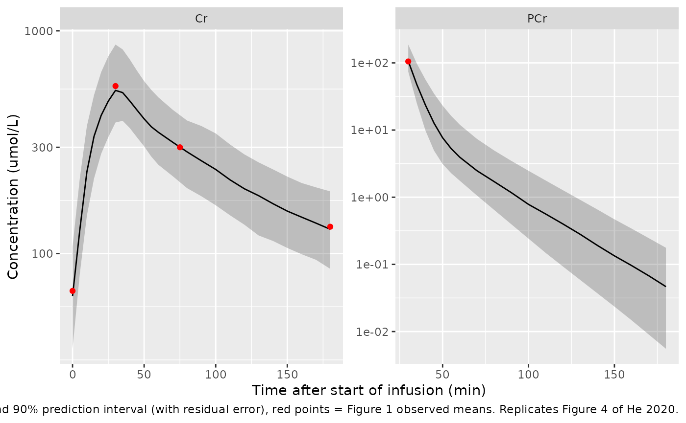
  )
Replicating Figure 5 (multiple-dose regimens)
Figure 5 shows the median of 1,000 simulated profiles per age group for four 4-day regimens: 30-min infusions q24h (regimen 1) or q12h (regimen 2), and 300-min (regimen 3) or 600-min (regimen 4) infusions q12h. The group weights used for the published simulation are not reported. Here each group is represented by a typical child at that group’s median weight in the virtual cohort, with eGFR at the reference value.
reg <- data.frame(
  regimen = paste("Regimen", 1:4),
  tau = c(1440, 720, 720, 720),
  dur = c(30, 30, 300, 600)
)
grp_typ <- cohort |>
  group_by(group) |>
  summarise(WT = median(WT), dose_g = first(dose_g)) |>
  mutate(CRCL = 127.78)
f5_grid <- seq(0, 8000, by = 2)
fig5 <- bind_rows(lapply(seq_len(nrow(reg)), function(r) {
  n_dose <- 4 * 1440 / reg$tau[r]
  subj <- grp_typ |> mutate(id = seq_len(n()))
  rxode2::rxSolve(
    mod_typ,
    make_events(subj, (seq_len(n_dose) - 1) * reg$tau[r], reg$dur[r], f5_grid),
    returnType = "data.frame"
  ) |>
    mutate(group = subj$group[id], regimen = reg$regimen[r])
}))
#> ℹ omega/sigma items treated as zero: 'etalcl', 'etalvc_creatine', 'etalvp_creatine', 'etalcl_creatine', 'etalrbase_creatine'
#> Warning: multi-subject simulation without without 'omega'
#> ℹ omega/sigma items treated as zero: 'etalcl', 'etalvc_creatine', 'etalvp_creatine', 'etalcl_creatine', 'etalrbase_creatine'
#> Warning: multi-subject simulation without without 'omega'
#> ℹ omega/sigma items treated as zero: 'etalcl', 'etalvc_creatine', 'etalvp_creatine', 'etalcl_creatine', 'etalrbase_creatine'
#> Warning: multi-subject simulation without without 'omega'
#> ℹ omega/sigma items treated as zero: 'etalcl', 'etalvc_creatine', 'etalvp_creatine', 'etalcl_creatine', 'etalrbase_creatine'
#> Warning: multi-subject simulation without without 'omega'
fig5 |>
  select(time, group, regimen, PCr = Cc, Cr = Cc_creatine) |>
  pivot_longer(c(PCr, Cr), names_to = "analyte", values_to = "conc") |>
  ggplot(aes(time, conc)) +
  geom_line() +
  facet_grid(regimen ~ group + analyte, scales = "free_y") +
  labs(
    x = "Time (min)", y = "Concentration (umol/L)",
    caption = "Typical-value profiles. Replicates Figure 5 of He 2020."
  ) +
  theme(strip.text = element_text(size = 6), axis.text = element_text(size = 6))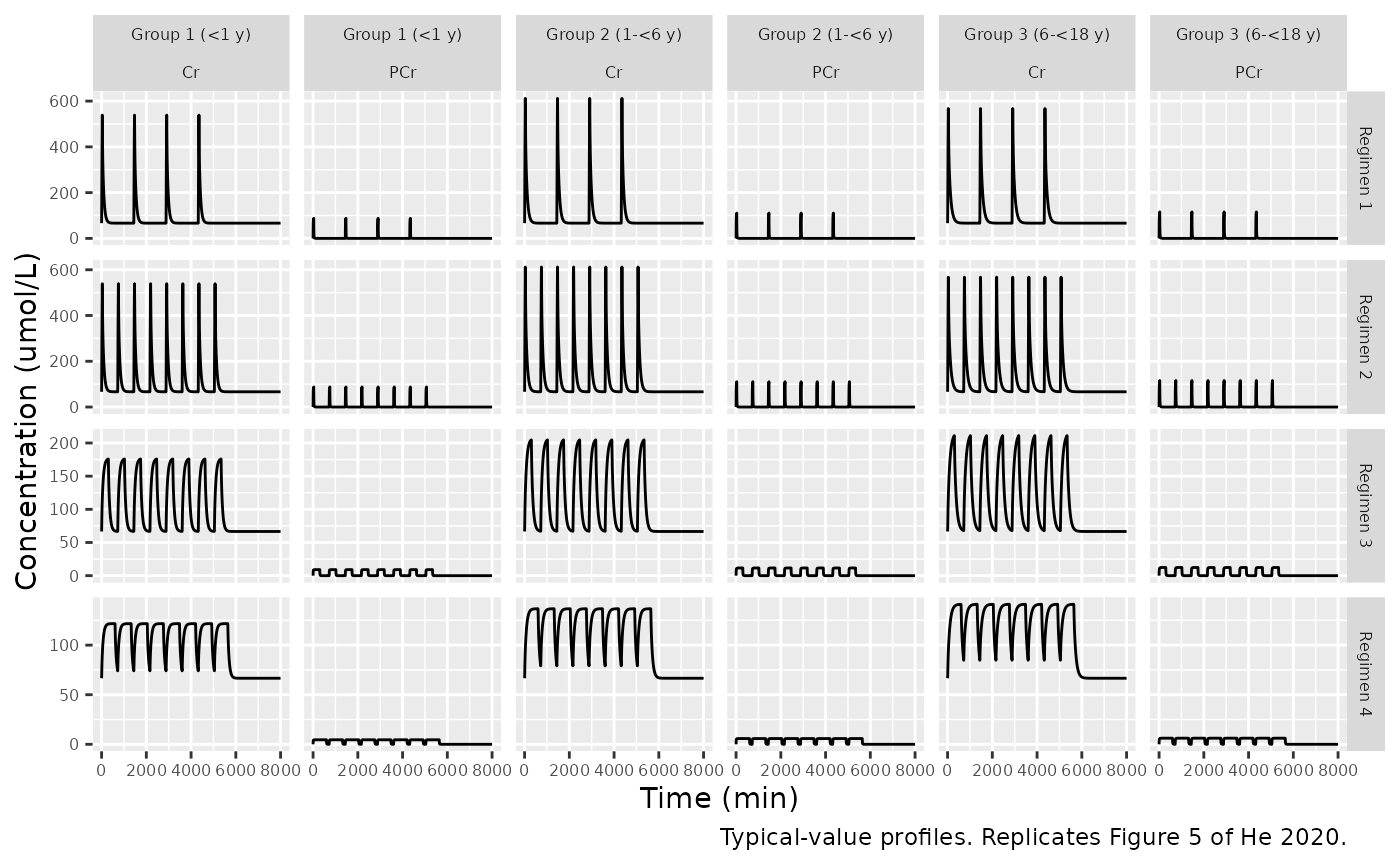
The paper’s text reports two things about these simulations. Under regimens 1 and 2, PCr is essentially gone within 3 h of the start of an infusion (median below 0.1 umol/L). Cr returns to its baseline of about 67 umol/L within 12 h.
f5_text <- fig5 |>
  filter(regimen %in% c("Regimen 1", "Regimen 2"), time %in% c(180, 720)) |>
  select(regimen, group, time, PCr = Cc, Cr = Cc_creatine, rbase = rbase_creatine)
knitr::kable(f5_text, digits = 3)| regimen | group | time | PCr | Cr | rbase |
|---|---|---|---|---|---|
| Regimen 1 | Group 1 (<1 y) | 180 | 0.008 | 102.021 | 66.6 |
| Regimen 1 | Group 1 (<1 y) | 720 | 0.000 | 66.606 | 66.6 |
| Regimen 1 | Group 2 (1-<6 y) | 180 | 0.026 | 122.627 | 66.6 |
| Regimen 1 | Group 2 (1-<6 y) | 720 | 0.000 | 66.632 | 66.6 |
| Regimen 1 | Group 3 (6-<18 y) | 180 | 0.078 | 140.827 | 66.6 |
| Regimen 1 | Group 3 (6-<18 y) | 720 | 0.000 | 66.776 | 66.6 |
| Regimen 2 | Group 1 (<1 y) | 180 | 0.008 | 102.021 | 66.6 |
| Regimen 2 | Group 1 (<1 y) | 720 | 0.000 | 66.606 | 66.6 |
| Regimen 2 | Group 2 (1-<6 y) | 180 | 0.026 | 122.627 | 66.6 |
| Regimen 2 | Group 2 (1-<6 y) | 720 | 0.000 | 66.632 | 66.6 |
| Regimen 2 | Group 3 (6-<18 y) | 180 | 0.078 | 140.827 | 66.6 |
| Regimen 2 | Group 3 (6-<18 y) | 720 | 0.000 | 66.776 | 66.6 |
stopifnot(
  all(f5_text$PCr[f5_text$time == 180] < 0.1),
  all(abs(f5_text$Cr[f5_text$time == 720] - f5_text$rbase[f5_text$time == 720]) < 1)
)
During the long infusions of regimens 3 and 4, both analytes approach
a plateau. At that plateau, the exogenous Cr to PCr ratio equals
Fm x CL_PCr / CL_Cr. This ratio is independent of weight
and dose, because both clearances carry the same allometric exponent, so
it can be checked against Figure 5 without knowing the group weights.
The Figure 5 plateaus were digitised by the maintainers from the regimen
4 panels.
plateau <- fig5 |>
  filter(regimen == "Regimen 4", time == 590) |>
  mutate(ratio = (Cc_creatine - rbase_creatine) / Cc)
fig5_digitised <- data.frame(
  group = grp_typ$group,
  PCr_plateau = c(4.85, 5.35, 7.3),
  Cr_plateau = c(127, 137, 157)
) |>
  mutate(fig5_ratio = (Cr_plateau - 67) / PCr_plateau)
cmp5 <- inner_join(select(plateau, group, PCr = Cc, Cr = Cc_creatine, ratio),
  fig5_digitised,
  by = "group"
)
knitr::kable(cmp5, digits = 2)| group | PCr | Cr | ratio | PCr_plateau | Cr_plateau | fig5_ratio |
|---|---|---|---|---|---|---|
| Group 1 (<1 y) | 4.55 | 121.65 | 12.09 | 4.85 | 127 | 12.37 |
| Group 2 (1-<6 y) | 5.80 | 136.68 | 12.09 | 5.35 | 137 | 13.08 |
| Group 3 (6-<18 y) | 6.17 | 141.15 | 12.08 | 7.30 | 157 | 12.33 |
stopifnot(
  abs(median(cmp5$ratio) - 0.75 * 1.33 / 0.0825) / (0.75 * 1.33 / 0.0825) < 0.05,
  abs(median(cmp5$fig5_ratio) / median(cmp5$ratio) - 1) < 0.10
)
The simulated plateau ratio is 12.1. The ratio read from the Figure 5
regimen 4 panels is 12.4. Agreement within 10% confirms the
mole-for-mole Fm coupling and the relative PCr and Cr
clearances. The absolute plateau heights also depend on the unreported
group weights.
PKNCA
The paper reports no NCA parameters, so the single-dose NCA below serves as a reference for users. It covers the stochastic cohort, one 30-min infusion per age group, for PCr and for baseline-subtracted (exogenous) Cr.
rxode2::rxSetSeed(20201116)
nca_grid <- c(0, 2, 5, 10, 15, 20, 25, 30, 32, 35, 40, 45, 50, 60, 75, 90, 120, 180, 240, 360, 480, 720)
nca_sim <- rxode2::rxSolve(
  mod, make_events(cohort, 0, 30, nca_grid),
  returnType = "data.frame"
) |>
  left_join(select(cohort, id, treatment = group), by = "id") |>
  mutate(Cr_exo = Cc_creatine - rbase_creatine)

dose_df <- cohort |>
  transmute(id, treatment = group, time = 0, amt = g_to_umol(dose_g))

run_nca <- function(conc_col) {
  conc_df <- nca_sim |>
    transmute(id, treatment, time, conc = .data[[conc_col]]) |>
    filter(!is.na(conc))
  conc_obj <- PKNCA::PKNCAconc(conc_df, conc ~ time | treatment + id)
  dose_obj <- PKNCA::PKNCAdose(dose_df, amt ~ time | treatment + id)
  intervals <- data.frame(
    start = 0, end = Inf, cmax = TRUE, tmax = TRUE,
    aucinf.obs = TRUE, half.life = TRUE
  )
  res <- PKNCA::pk.nca(PKNCA::PKNCAdata(conc_obj, dose_obj, intervals = intervals))
  as.data.frame(summary(res)) |> mutate(analyte = conc_col)
}
nca_pcr <- run_nca("Cc")
#> Warning in assert_conc(conc, any_missing_conc = any_missing_conc): Negative
#> concentrations found
#> Warning in assert_conc(conc = conc): Negative concentrations found
#> Warning in assert_conc(conc, any_missing_conc = any_missing_conc): Negative
#> concentrations found
#> Warning in assert_conc(conc, any_missing_conc = any_missing_conc): Negative
#> concentrations found
#> Warning in assert_conc(conc, any_missing_conc = any_missing_conc): Negative
#> concentrations found
#> Warning in assert_conc(conc, any_missing_conc = any_missing_conc): Negative
#> concentrations found
#> Warning in assert_conc(conc, any_missing_conc = any_missing_conc): Negative
#> concentrations found
#> Warning in log(data$conc): NaNs produced
#> Warning in assert_conc(conc, any_missing_conc = any_missing_conc): Negative
#> concentrations found
#> Warning in log(conc.2/conc.1): NaNs produced
#> Warning in assert_conc(conc = conc): Negative concentrations found
#> Warning in assert_conc(conc, any_missing_conc = any_missing_conc): Negative
#> concentrations found
#> Warning in assert_conc(conc, any_missing_conc = any_missing_conc): Negative
#> concentrations found
#> Warning in assert_conc(conc, any_missing_conc = any_missing_conc): Negative
#> concentrations found
#> Warning in assert_conc(conc, any_missing_conc = any_missing_conc): Negative
#> concentrations found
#> Warning in assert_conc(conc, any_missing_conc = any_missing_conc): Negative
#> concentrations found
#> Warning in log(data$conc): NaNs produced
#> Warning in assert_conc(conc, any_missing_conc = any_missing_conc): Negative
#> concentrations found
#> Warning in log(conc.2/conc.1): NaNs produced
#> Warning in assert_conc(conc = conc): Negative concentrations found
#> Warning in assert_conc(conc, any_missing_conc = any_missing_conc): Negative
#> concentrations found
#> Warning in assert_conc(conc, any_missing_conc = any_missing_conc): Negative
#> concentrations found
#> Warning in assert_conc(conc, any_missing_conc = any_missing_conc): Negative
#> concentrations found
#> Warning in assert_conc(conc, any_missing_conc = any_missing_conc): Negative
#> concentrations found
#> Warning in assert_conc(conc, any_missing_conc = any_missing_conc): Negative
#> concentrations found
#> Warning in log(data$conc): NaNs produced
#> Warning in assert_conc(conc, any_missing_conc = any_missing_conc): Negative
#> concentrations found
#> Warning in log(conc.2/conc.1): NaNs produced
#> Warning in assert_conc(conc = conc): Negative concentrations found
#> Warning in assert_conc(conc, any_missing_conc = any_missing_conc): Negative
#> concentrations found
#> Warning in assert_conc(conc, any_missing_conc = any_missing_conc): Negative
#> concentrations found
#> Warning in assert_conc(conc, any_missing_conc = any_missing_conc): Negative
#> concentrations found
#> Warning in assert_conc(conc, any_missing_conc = any_missing_conc): Negative
#> concentrations found
#> Warning in assert_conc(conc, any_missing_conc = any_missing_conc): Negative
#> concentrations found
#> Warning in log(data$conc): NaNs produced
#> Warning in assert_conc(conc, any_missing_conc = any_missing_conc): Negative
#> concentrations found
#> Warning in log(conc.2/conc.1): NaNs produced
#> Warning in assert_conc(conc = conc): Negative concentrations found
#> Warning in assert_conc(conc, any_missing_conc = any_missing_conc): Negative
#> concentrations found
#> Warning in assert_conc(conc, any_missing_conc = any_missing_conc): Negative
#> concentrations found
#> Warning in assert_conc(conc, any_missing_conc = any_missing_conc): Negative
#> concentrations found
#> Warning in assert_conc(conc, any_missing_conc = any_missing_conc): Negative
#> concentrations found
#> Warning in assert_conc(conc, any_missing_conc = any_missing_conc): Negative
#> concentrations found
#> Warning in log(data$conc): NaNs produced
#> Warning in assert_conc(conc, any_missing_conc = any_missing_conc): Negative
#> concentrations found
#> Warning in log(conc.2/conc.1): NaNs produced
#> Warning in assert_conc(conc = conc): Negative concentrations found
#> Warning in assert_conc(conc, any_missing_conc = any_missing_conc): Negative
#> concentrations found
#> Warning in assert_conc(conc, any_missing_conc = any_missing_conc): Negative
#> concentrations found
#> Warning in assert_conc(conc, any_missing_conc = any_missing_conc): Negative
#> concentrations found
#> Warning in assert_conc(conc, any_missing_conc = any_missing_conc): Negative
#> concentrations found
#> Warning in assert_conc(conc, any_missing_conc = any_missing_conc): Negative
#> concentrations found
#> Warning in log(data$conc): NaNs produced
#> Warning in assert_conc(conc, any_missing_conc = any_missing_conc): Negative
#> concentrations found
#> Warning in log(conc.2/conc.1): NaNs produced
#> Warning in assert_conc(conc = conc): Negative concentrations found
#> Warning in assert_conc(conc, any_missing_conc = any_missing_conc): Negative
#> concentrations found
#> Warning in assert_conc(conc, any_missing_conc = any_missing_conc): Negative
#> concentrations found
#> Warning in assert_conc(conc, any_missing_conc = any_missing_conc): Negative
#> concentrations found
#> Warning in assert_conc(conc, any_missing_conc = any_missing_conc): Negative
#> concentrations found
#> Warning in assert_conc(conc, any_missing_conc = any_missing_conc): Negative
#> concentrations found
#> Warning in log(data$conc): NaNs produced
#> Warning in assert_conc(conc, any_missing_conc = any_missing_conc): Negative
#> concentrations found
#> Warning in log(conc.2/conc.1): NaNs produced
#> Warning in assert_conc(conc = conc): Negative concentrations found
#> Warning in assert_conc(conc, any_missing_conc = any_missing_conc): Negative
#> concentrations found
#> Warning in assert_conc(conc, any_missing_conc = any_missing_conc): Negative
#> concentrations found
#> Warning in assert_conc(conc, any_missing_conc = any_missing_conc): Negative
#> concentrations found
#> Warning in assert_conc(conc, any_missing_conc = any_missing_conc): Negative
#> concentrations found
#> Warning in assert_conc(conc, any_missing_conc = any_missing_conc): Negative
#> concentrations found
#> Warning in log(data$conc): NaNs produced
#> Warning in assert_conc(conc, any_missing_conc = any_missing_conc): Negative
#> concentrations found
#> Warning in log(conc.2/conc.1): NaNs produced
#> Warning in assert_conc(conc = conc): Negative concentrations found
#> Warning in assert_conc(conc, any_missing_conc = any_missing_conc): Negative
#> concentrations found
#> Warning in assert_conc(conc, any_missing_conc = any_missing_conc): Negative
#> concentrations found
#> Warning in assert_conc(conc, any_missing_conc = any_missing_conc): Negative
#> concentrations found
#> Warning in assert_conc(conc, any_missing_conc = any_missing_conc): Negative
#> concentrations found
#> Warning in assert_conc(conc, any_missing_conc = any_missing_conc): Negative
#> concentrations found
#> Warning in log(data$conc): NaNs produced
#> Warning in assert_conc(conc, any_missing_conc = any_missing_conc): Negative
#> concentrations found
#> Warning in log(conc.2/conc.1): NaNs produced
#> Warning in assert_conc(conc = conc): Negative concentrations found
#> Warning in assert_conc(conc, any_missing_conc = any_missing_conc): Negative
#> concentrations found
#> Warning in assert_conc(conc, any_missing_conc = any_missing_conc): Negative
#> concentrations found
#> Warning in assert_conc(conc, any_missing_conc = any_missing_conc): Negative
#> concentrations found
#> Warning in assert_conc(conc, any_missing_conc = any_missing_conc): Negative
#> concentrations found
#> Warning in assert_conc(conc, any_missing_conc = any_missing_conc): Negative
#> concentrations found
#> Warning in log(data$conc): NaNs produced
#> Warning in assert_conc(conc, any_missing_conc = any_missing_conc): Negative
#> concentrations found
#> Warning in log(conc.2/conc.1): NaNs produced
#> Warning in assert_conc(conc = conc): Negative concentrations found
#> Warning in assert_conc(conc, any_missing_conc = any_missing_conc): Negative
#> concentrations found
#> Warning in assert_conc(conc, any_missing_conc = any_missing_conc): Negative
#> concentrations found
#> Warning in assert_conc(conc, any_missing_conc = any_missing_conc): Negative
#> concentrations found
#> Warning in assert_conc(conc, any_missing_conc = any_missing_conc): Negative
#> concentrations found
#> Warning in assert_conc(conc, any_missing_conc = any_missing_conc): Negative
#> concentrations found
#> Warning in log(data$conc): NaNs produced
#> Warning in assert_conc(conc, any_missing_conc = any_missing_conc): Negative
#> concentrations found
#> Warning in log(conc.2/conc.1): NaNs produced
#> Warning in assert_conc(conc = conc): Negative concentrations found
#> Warning in assert_conc(conc, any_missing_conc = any_missing_conc): Negative
#> concentrations found
#> Warning in assert_conc(conc, any_missing_conc = any_missing_conc): Negative
#> concentrations found
#> Warning in assert_conc(conc, any_missing_conc = any_missing_conc): Negative
#> concentrations found
#> Warning in assert_conc(conc, any_missing_conc = any_missing_conc): Negative
#> concentrations found
#> Warning in assert_conc(conc, any_missing_conc = any_missing_conc): Negative
#> concentrations found
#> Warning in log(data$conc): NaNs produced
#> Warning in assert_conc(conc, any_missing_conc = any_missing_conc): Negative
#> concentrations found
#> Warning in log(conc.2/conc.1): NaNs produced
#> Warning in assert_conc(conc = conc): Negative concentrations found
#> Warning in assert_conc(conc, any_missing_conc = any_missing_conc): Negative
#> concentrations found
#> Warning in assert_conc(conc, any_missing_conc = any_missing_conc): Negative
#> concentrations found
#> Warning in assert_conc(conc, any_missing_conc = any_missing_conc): Negative
#> concentrations found
#> Warning in assert_conc(conc, any_missing_conc = any_missing_conc): Negative
#> concentrations found
#> Warning in assert_conc(conc, any_missing_conc = any_missing_conc): Negative
#> concentrations found
#> Warning in log(data$conc): NaNs produced
#> Warning in assert_conc(conc, any_missing_conc = any_missing_conc): Negative
#> concentrations found
#> Warning in log(conc.2/conc.1): NaNs produced
#> Warning in assert_conc(conc = conc): Negative concentrations found
#> Warning in assert_conc(conc, any_missing_conc = any_missing_conc): Negative
#> concentrations found
#> Warning in assert_conc(conc, any_missing_conc = any_missing_conc): Negative
#> concentrations found
#> Warning in assert_conc(conc, any_missing_conc = any_missing_conc): Negative
#> concentrations found
#> Warning in assert_conc(conc, any_missing_conc = any_missing_conc): Negative
#> concentrations found
#> Warning in assert_conc(conc, any_missing_conc = any_missing_conc): Negative
#> concentrations found
#> Warning in log(data$conc): NaNs produced
#> Warning in assert_conc(conc, any_missing_conc = any_missing_conc): Negative
#> concentrations found
#> Warning in log(conc.2/conc.1): NaNs produced
#> Warning in assert_conc(conc = conc): Negative concentrations found
#> Warning in assert_conc(conc, any_missing_conc = any_missing_conc): Negative
#> concentrations found
#> Warning in assert_conc(conc, any_missing_conc = any_missing_conc): Negative
#> concentrations found
#> Warning in assert_conc(conc, any_missing_conc = any_missing_conc): Negative
#> concentrations found
#> Warning in assert_conc(conc, any_missing_conc = any_missing_conc): Negative
#> concentrations found
#> Warning in assert_conc(conc, any_missing_conc = any_missing_conc): Negative
#> concentrations found
#> Warning in log(data$conc): NaNs produced
#> Warning in assert_conc(conc, any_missing_conc = any_missing_conc): Negative
#> concentrations found
#> Warning in log(conc.2/conc.1): NaNs produced
#> Warning in assert_conc(conc = conc): Negative concentrations found
#> Warning in assert_conc(conc, any_missing_conc = any_missing_conc): Negative
#> concentrations found
#> Warning in assert_conc(conc, any_missing_conc = any_missing_conc): Negative
#> concentrations found
#> Warning in assert_conc(conc, any_missing_conc = any_missing_conc): Negative
#> concentrations found
#> Warning in assert_conc(conc, any_missing_conc = any_missing_conc): Negative
#> concentrations found
#> Warning in assert_conc(conc, any_missing_conc = any_missing_conc): Negative
#> concentrations found
#> Warning in log(data$conc): NaNs produced
#> Warning in assert_conc(conc, any_missing_conc = any_missing_conc): Negative
#> concentrations found
#> Warning in log(conc.2/conc.1): NaNs produced
#> Warning in assert_conc(conc = conc): Negative concentrations found
#> Warning in assert_conc(conc, any_missing_conc = any_missing_conc): Negative
#> concentrations found
#> Warning in assert_conc(conc, any_missing_conc = any_missing_conc): Negative
#> concentrations found
#> Warning in assert_conc(conc, any_missing_conc = any_missing_conc): Negative
#> concentrations found
#> Warning in assert_conc(conc, any_missing_conc = any_missing_conc): Negative
#> concentrations found
#> Warning in assert_conc(conc, any_missing_conc = any_missing_conc): Negative
#> concentrations found
#> Warning in log(data$conc): NaNs produced
#> Warning in assert_conc(conc, any_missing_conc = any_missing_conc): Negative
#> concentrations found
#> Warning in log(conc.2/conc.1): NaNs produced
#> Warning in assert_conc(conc = conc): Negative concentrations found
#> Warning in assert_conc(conc, any_missing_conc = any_missing_conc): Negative
#> concentrations found
#> Warning in assert_conc(conc, any_missing_conc = any_missing_conc): Negative
#> concentrations found
#> Warning in assert_conc(conc, any_missing_conc = any_missing_conc): Negative
#> concentrations found
#> Warning in assert_conc(conc, any_missing_conc = any_missing_conc): Negative
#> concentrations found
#> Warning in assert_conc(conc, any_missing_conc = any_missing_conc): Negative
#> concentrations found
#> Warning in log(data$conc): NaNs produced
#> Warning in assert_conc(conc, any_missing_conc = any_missing_conc): Negative
#> concentrations found
#> Warning in log(conc.2/conc.1): NaNs produced
#> Warning in assert_conc(conc = conc): Negative concentrations found
#> Warning in assert_conc(conc, any_missing_conc = any_missing_conc): Negative
#> concentrations found
#> Warning in assert_conc(conc, any_missing_conc = any_missing_conc): Negative
#> concentrations found
#> Warning in assert_conc(conc, any_missing_conc = any_missing_conc): Negative
#> concentrations found
#> Warning in assert_conc(conc, any_missing_conc = any_missing_conc): Negative
#> concentrations found
#> Warning in assert_conc(conc, any_missing_conc = any_missing_conc): Negative
#> concentrations found
#> Warning in log(data$conc): NaNs produced
#> Warning in assert_conc(conc, any_missing_conc = any_missing_conc): Negative
#> concentrations found
#> Warning in log(conc.2/conc.1): NaNs produced
nca_cr <- run_nca("Cr_exo")
bind_rows(nca_pcr, nca_cr) |>
  mutate(analyte = recode(analyte, Cc = "PCr", Cr_exo = "Cr (exogenous)")) |>
  select(analyte, treatment, N, cmax, tmax, half.life, aucinf.obs) |>
  rename(
    "Analyte" = analyte, "Age group" = treatment,
    "Cmax (umol/L)" = cmax, "Tmax (min)" = tmax, "t1/2 (min)" = half.life,
    "AUC0-inf (umol*min/L)" = aucinf.obs
  ) |>
knitr::kable(caption = "Single-dose NCA (geometric mean [CV]; Tmax median [range]).")| Analyte | Age group | N | Cmax (umol/L) | Tmax (min) | t1/2 (min) | AUC0-inf (umol*min/L) |
|---|---|---|---|---|---|---|
| PCr | Group 1 (<1 y) | 12 | 77.9 [19.2] | 30.0 [30.0, 30.0] | 15.2 [1.01] | 2500 [20.2], n=8 |
| PCr | Group 2 (1-<6 y) | 40 | 114 [22.9] | 30.0 [30.0, 30.0] | 17.1 [1.22] | 3540 [23.4], n=27 |
| PCr | Group 3 (6-<18 y) | 48 | 111 [26.9] | 30.0 [30.0, 30.0] | 20.9 [1.72] | 3550 [28.4], n=46 |
| Cr (exogenous) | Group 1 (<1 y) | 12 | 445 [15.5] | 32.0 [30.0, 35.0] | 46.8 [10.6] | 32400 [17.3] |
| Cr (exogenous) | Group 2 (1-<6 y) | 40 | 553 [26.6] | 32.0 [30.0, 35.0] | 53.9 [11.3] | 44500 [22.8] |
| Cr (exogenous) | Group 3 (6-<18 y) | 48 | 476 [32.4] | 32.0 [32.0, 40.0] | 65.8 [14.5] | 44500 [29.4] |
The PCr AUC0-inf is missing for some children because PKNCA could not fit an acceptable terminal slope to the very low concentrations of PCr’s slow peripheral-return phase. The Cr columns are baseline-subtracted.
Assumptions and deviations
- Dose molar conversion. The paper states doses in grams of phosphocreatine sodium and concentrations in umol/L without giving the molecular weight used. This vignette uses the anhydrous disodium salt (255.08 g/mol). That is the conventional labelled strength, and it is the only one of the three candidate salt forms that reproduces the Figure 1 means within 20%. The model itself is in umol and does not depend on the choice.
- Figure 1 and Figure 5 values are the maintainers’ digitisations of the published raster figures.
- Virtual cohort. Table 1 gives only overall medians and ranges. The age-band sizes, weight-for-age curve, weight scatter and eGFR CV are assumptions chosen to match the reported medians. Race is not reported.
- PCr below the LLOQ was handled with the M3 method in the fit. The model simulates the underlying concentration and has no censoring.
-
Maturation (Methods Eq. 5) was tested and rejected
by the authors, so it is not part of the model. Age is recorded under
covariatesDataExcluded. - PCr baseline. Endogenous plasma PCr was below the LLOQ before dosing in every child and was fixed to 0, as in the paper. The endogenous Cr baseline is a constant added to the drug-derived Cr concentration (Eq. 16). The model has no endogenous synthesis or turnover term.
- Fm = 0.75 is an assumption the authors carried from animal data (Xu et al., 2014). They report that fixing it at 0.5 or 1 barely changed the PCr parameters, but it scales the Cr volumes and clearances.