Regorafenib with M-2 and M-5 metabolites and enterohepatic circulation (Keunecke 2020)
Source:vignettes/articles/Keunecke_2020_regorafenib.Rmd
Keunecke_2020_regorafenib.RmdModel and source
Keunecke 2020 developed the model in two stages, on two different
cohorts, and this paper therefore contributes two model
files to nlmixr2lib.
mod_p1 <- rxode2::rxode(readModelDb("Keunecke_2020_regorafenib_phase1"))
mod_p3 <- rxode2::rxode(readModelDb("Keunecke_2020_regorafenib_phase3"))- Citation: Keunecke A, Hoefman S, Drenth H-J, Zisowsky J, Cleton A, Ploeger BA. Population pharmacokinetics of regorafenib in solid tumours: Exposure in clinical practice considering enterohepatic circulation and food intake. Br J Clin Pharmacol. 2020;86(12):2362-2376. doi:10.1111/bcp.14334.
- Article: https://doi.org/10.1111/bcp.14334
- Supplement (Appendix Sections 1-3, Tables A1-A2, Figures A1-A2): https://pmc.ncbi.nlm.nih.gov/articles/PMC7688542/
| Model file | Fitted to | Source table |
|---|---|---|
Keunecke_2020_regorafenib_phase1 |
62 patients, densely sampled, 2 phase 1 studies | Table 2 |
Keunecke_2020_regorafenib_phase3 |
906 patients, sparsely sampled, 4 phase 3 studies; adds the retained covariates | Table 3 |
The phase 1 parent-only model (Table 1) is not shipped separately: it is a development step whose parameters are carried into the phase 1 parent-metabolite model as fixed values, so Table 2 contains all of it.
Description of the final model:
Final joint parent + metabolite population PK model for oral regorafenib and its two pharmacologically active metabolites M-2 (N-oxide, BAY 75-7495) and M-5 (N-oxide N-desmethyl, BAY 81-8752), fitted to sparsely sampled data from four phase 3 studies in metastatic colorectal cancer, gastrointestinal stromal tumour and hepatocellular carcinoma (Keunecke 2020 Table 3). Structure is identical to the phase 1 model (Keunecke_2020_regorafenib_phase1): each analyte has a two-compartment disposition plus a gallbladder reservoir giving enterohepatic circulation, released during three 30-minute post-prandial windows per day; M-2 is formed pre-systemically through its own three-transit absorption chain and M-5 systemically from parent clearance. This version adds the retained covariate effects - sex and body mass index on parent clearance, and sex on both metabolite clearances - with women having lower clearance of all three analytes. Because the metabolite clearance random effects were almost perfectly correlated, the authors reduced the model to a single shared metabolite eta rescaled by a factor, so M-5 uses the M-2 eta multiplied by sd_ratio_cl_m5. The parent disposition is tabulated as the composites CL_P/(1-FRM2), VC_P/(1-FRM2), Q_P/(1-FRM2) and VP_P/(1-FRM2) and is rescaled by (1 - fm_m2) in model() to recover CL_P, VC_P, Q_P and VP_P, which the metabolites inherit; all values remain apparent, relative to oral bioavailability.
Structure
Regorafenib is an oral multikinase inhibitor whose two major metabolites, M-2 (N-oxide, BAY 75-7495) and M-5 (N-oxide N-desmethyl, BAY 81-8752), are pharmacologically active and reach concentrations close to the parent at steady state. All three analytes undergo enterohepatic circulation (EHC) through the gallbladder, which the authors identified as a significant disposition pathway.
Per Figure 1 of the paper:
- The dose leaves a depot at rate
kaand splits there: a fractionfm_m2enters a three-transit chain that forms M-2 pre-systemically, and1 - fm_m2enters a two-transit chain feeding the parent central compartment. - Each analyte has a two-compartment disposition plus a
gallbladder reservoir. Drug leaves the central compartment for
the gallbladder at a constant first-order rate
kbm(the paper’sk_CG), independent of food. - Release back to the central compartment is gated by food
intake: it happens only during the
dge= 0.5 h window after each of three daily meals, and is then essentially instantaneous (kehc= 100 1/h). This is the “Not during meal” / “During meal” pair of ODE systems in the Figure 1 caption. - M-5 is formed systemically, as the fraction
fm_m5of parent clearance leaving the parent central compartment.
Because no intravenous or direct-metabolite data existed, the metabolite volumes, inter-compartmental flow and gallbladder rate constants are fixed to the parent values, and every volume and clearance is apparent.
One bookkeeping point matters for the metabolites. Tables 2 and 3
tabulate the parent disposition parameters as the composites
CL_P/(1-FRM2), VC_P/(1-FRM2),
Q_P/(1-FRM2) and VP_P/(1-FRM2), so
model() multiplies each by (1 - fm_m2) to
recover CL_P, VC_P, Q_P and
VP_P themselves - which are what the metabolites then
inherit. The parent profile is unchanged by this (the factor cancels in
every parent-only ratio), but the metabolite exposures are not; see item
3 of Assumptions and deviations.
Population
The phase 1 model was fitted to 62 patients with advanced solid tumours from two studies: 14814 (NCT01339104, USA, n = 44, 774 PK observations, sampled at cycle 1 day 21 predose to 24 h post-dose) and 15823 (NCT02398513, Mainland China, n = 18, 566 observations, cycle 0 day 1 and cycle 1 day 21, predose to 96 h post-dose).
The phase 3 model was fitted to 906 patients from four pivotal placebo-controlled studies (Appendix Table A1): CORRECT (n = 388, metastatic colorectal carcinoma), GRID (n = 81, gastrointestinal stromal tumour), CONCUR (n = 98, metastatic colorectal carcinoma, Asia) and RESORCE (n = 339, hepatocellular carcinoma after sorafenib). Sampling was sparse - a predose trough at cycle 1 day 15 and cycle 2 day 15 for most patients, with 2-4 h and 5-10 h post-dose samples in subsets. Combined, the full dataset is 968 patients and 10,019 observations, all at a 160 mg once-daily starting dose on a 3-weeks-on / 1-week-off schedule.
Baseline characteristics of the phase 3 cohort (Appendix Table A2, Total column): median age 61 years (5th-95th percentile 40-78), median body weight 70 kg (48-99), median BMI 24.5 kg/m^2 (18.5-32.4), 27.9% female, 54.4% Caucasian and 33.8% Asian, tumour type 54% CRC / 8.8% GIST / 37.2% HCC, median eGFR 100 mL/min/1.73m^2 and median albumin 4.0 g/dL.
str(readModelDb("Keunecke_2020_regorafenib_phase3")()$population)
#> List of 16
#>  $ species         : chr "human"
#>  $ n_subjects      : int 906
#>  $ n_studies       : int 4
#>  $ age_range       : chr "40-78 years (5th-95th percentile)"
#>  $ age_median      : chr "61 years"
#>  $ weight_range    : chr "48-99 kg (5th-95th percentile)"
#>  $ weight_median   : chr "70 kg"
#>  $ bmi_range       : chr "18.5-32.4 kg/m^2 (5th-95th percentile)"
#>  $ bmi_median      : chr "24.5 kg/m^2"
#>  $ sex_female_pct  : num 27.9
#>  $ race_ethnicity  : Named num [1:6] 54.4 33.8 1.1 0.1 0.2 10.4
#>   ..- attr(*, "names")= chr [1:6] "Caucasian" "Asian" "Black" "AmericanIndian" ...
#>  $ disease_state   : chr "Adults with treatment-refractory metastatic colorectal carcinoma (54%), advanced gastrointestinal stromal tumou"| __truncated__
#>  $ dose_range      : chr "Regorafenib 160 mg once daily (4 x 40 mg tablets), 3 weeks on / 1 week off, versus matching placebo."
#>  $ regions         : chr "North America, Europe, Israel, Australia, South America and Asia."
#>  $ hepatic_function: chr "Category A (normal) 56.4%, B1 28.7%, B2 11.7%, C 3.2% (Appendix Table A2 footnote, defined on total bilirubin and AST/ALT)."
#>  $ notes           : chr "Keunecke 2020 Appendix Tables A1 and A2. The four phase 3 studies are CORRECT (14387, NCT01103323, n = 388, 405"| __truncated__
Source trace
Every ini() entry in both model files carries an in-file
comment naming its source row. Collected here:
| Equation / parameter | Phase 1 value (Table 2) | Phase 3 value (Table 3) | Source location |
|---|---|---|---|
lka |
0.482 1/h, Fixed | 0.482 1/h, Fixed | Table 2 / 3 row “k a, h-1”; section 2.3.1 |
| number of transit compartments | 2 (parent), 3 (M-2) | same | Figure 1 schematic; section 3.1 “required two transition compartments” |
logitfm_m2 |
-0.355 (RSE 26.7%) | -0.355, Fixed | Table 2 / 3 row “FRM2”; footnote “corresponds with 41%” |
logitfm_m5 |
-1.09 (RSE 19.4%) | -1.09, Fixed | Table 2 / 3 row “FRM5”; footnote “corresponds with 25%” |
lcl |
4.02 L/h, Fixed | 3.05 L/h, Fixed | Table 2 / 3 row “CL P /(1-FRM2)”; section 3.3.1 |
lvc |
10.7 L, Fixed | 10.7 L, Fixed | Table 2 / 3 row “VC P /(1-FRM2)” |
lq |
11.0 L/h, Fixed | 11.0 L/h, Fixed | Table 2 / 3 row “Q P /(1-FRM2)” |
lvp |
162 L, Fixed | 162 L, Fixed | Table 2 / 3 row “VP P /(1-FRM2)” |
lkbm (paper k_CG) |
0.141 1/h, Fixed | 0.141 1/h, Fixed | Table 2 / 3 row “k CG, h-1” |
lkehc (paper k_GE) |
100 1/h, Fixed | 100 1/h, Fixed | Table 2 / 3 row “k GE, h-1”; section 2.3.1 |
tmeal1 / tmeal2 / tmeal3
|
8 / 12 / 18 h, Fixed | same | Table 2 / 3 rows “Breakfast / Lunch / Dinner, h”; section 2.2 |
dge |
0.5 h, Fixed | 0.5 h, Fixed | Table 2 / 3 row “DGE, h”; section 2.3.1 “approximately 30 min” |
lcl_m2 |
2.45 L/h (RSE 4.98%) | 1.99 L/h (RSE 0.255%) | Table 2 / 3 row “CL M-2” |
lcl_m5 |
0.746 L/h (RSE 28.8%) | 1.42 L/h (RSE 3.76%) | Table 2 / 3 row “CL M-5” |
e_sexf_cl |
n/a | 0.169, Fixed | Table 3 row “Sex on regorafenib clearance”; Appendix Section 3.1 |
e_bmi_cl |
n/a | -0.363, Fixed | Table 3 row “BMI on regorafenib clearance”; Appendix Section 3.1 |
e_sexf_cl_m2 |
n/a | 0.380 (RSE 5.06%) | Table 3 row “Sex on M-2 clearance” |
e_sexf_cl_m5 |
n/a | 0.761 (RSE 5.08%) | Table 3 row “Sex on M-5 clearance” |
sd_ratio_cl_m5 |
n/a | 2.21 (RSE 3.41%) | Table 3 row “Factor IIV CL M-5”; Appendix Section 3.3 |
etalka |
0.127, Fixed | 0.127, Fixed | Table 2 / 3 row “omega^2 k a” |
etalcl |
0.117 | 0.189 | Table 2 / 3 row “omega^2 CL P” |
etalcl_m2 |
0.267 | 0.385 | Table 2 / 3 row “omega^2 CL M-2” |
etalcl_m5 |
1.95 | derived as sd_ratio_cl_m5 * etalcl_m2
|
Table 2 row “omega^2 CL M-5”; Appendix Section 3.3 |
| eta covariances | 0.122 / 0.157 / 0.656 | 0.206 | Table 2 rows “omega CL P,CL M-2” etc.; Table 3 row “omega CL P, CL M-2/M-5” |
etalogitfm_m2 |
0.156 | 0.156, Fixed | Table 2 / 3 row “omega^2 FRM2” |
etalogitfm_m5 |
0.841 | 0.841, Fixed | Table 2 / 3 row “omega^2 FRM5” |
propSd |
0.406 | 0.543 | Table 2 / 3 row “Parent Prop. error, SD” |
addSd_m2 / propSd_m2
|
0.001 Fixed / 0.380 | 0.001 Fixed / 0.485 | Table 2 / 3 rows “M-2 Add./Prop. error, SD” |
addSd_m5 / propSd_m5
|
0.001 Fixed / 0.455 | 0.001 Fixed / 1.14 | Table 2 / 3 rows “M-5 Add./Prop. error, SD” |
| parent central / gallbladder / peripheral ODEs | n/a | n/a | Figure 1 caption, “Not during meal” and “During meal” equation pairs |
dose split ka * FRM2 vs ka * (1-FRM2)
|
n/a | n/a | Figure 1 schematic |
M-5 formation CL_Parent * FRM5
|
n/a | n/a | Figure 1 schematic |
| unbound fractions 0.5% / 0.2% / 0.05% | n/a | n/a | Introduction, paragraph 3 (used only for the Figure 4B reconstruction below) |
Event tables
t in the model is absolute time and the meal switch
reads a time of day, so the event table origin must be
midnight. Two consequences drive the helper below.
- Doses go in at the protocol clock time: 08:30 for phase 1 (breakfast 08:00 plus the protocol’s 0.5 h) and 09:00 for phase 3 (breakfast 1 h before the dose, the interval that minimised the objective function in section 3.3.1).
- The gallbladder empties over a 0.5 h window with a rate constant of 100 1/h. That is a stiff, short-lived discontinuity, and a solver left to choose its own steps over a multi-week run-in will step straight over it and fail with “could not solve the system”. Every meal-window edge therefore gets an explicit record so the solver is forced to stop there.
MEAL_EDGES <- c(8, 8.5, 12, 12.5, 18, 18.5)  # tmeal* and tmeal* + dge

# Build an event table for one subject: `ndays` once-daily 160 mg doses at
# clock time `dose_t`, meal-edge stops throughout, and observations on the
# ODE state `central` over `obs_times` (absolute hours from midnight, day 1).
make_subject <- function(id, dose_t, ndays, obs_times, dose_mg = 160, ...) {
  day <- 24 * (0:(ndays - 1))
  doses <- data.frame(time = dose_t + day, amt = dose_mg, evid = 1L,
                      cmt = "depot", dvid = NA_integer_)
  stops <- sort(unique(c(outer(day, MEAL_EDGES, "+"))))
  obs <- data.frame(time = sort(unique(c(stops, obs_times))), amt = NA_real_,
                    evid = 0L, cmt = "central", dvid = 1L)
  out <- rbind(doses, obs)
  out$id <- id
  extra <- list(...)
  for (nm in names(extra)) out[[nm]] <- extra[[nm]]
  out[order(out$time, -out$evid), ]
}
Observation rows use cmt = "central" (an actual ODE
state) and dvid = 1L. The model has three endpoints whose
observables read from three different ODE states; rxSolve
still returns Cc, Cc_m2 and Cc_m5
as columns on every observation row, and solving
$simulationModel rather than the rxUi object
keeps the endpoint states from being misclassified as input
parameters.
Enterohepatic circulation is what shapes the profile
Section 3.1 attributes to EHC “the observed higher steady state concentration caused by gallbladder emptying and rapid reabsorption, followed by a rapid decrease after dosing through distribution and elimination, and subsequent slow absorption step 3-4 h later”. Appendix Figure A1 shows the same thing per patient, with the gallbladder-emptying windows shaded.
Below, the same typical phase 1 patient is simulated with EHC as
published and with the central-to-gallbladder transfer switched off
(kbm set to effectively zero), over day 21 of once-daily
dosing.
obs_day21 <- seq(20 * 24, 21 * 24, by = 0.02)
ev_typ_p1 <- make_subject(1L, dose_t = 8.5, ndays = 21, obs_times = obs_day21)

solve_typ <- function(mod, ev, ...) {
  rxode2::rxSolve(rxode2::zeroRe(mod)$simulationModel, ev,
                  returnType = "data.frame", atol = 1e-10, rtol = 1e-8, ...)
}

sim_ehc  <- solve_typ(mod_p1, ev_typ_p1)
#> ℹ omega/sigma items treated as zero: 'etalka', 'etalcl', 'etalcl_m2', 'etalcl_m5', 'etalogitfm_m2', 'etalogitfm_m5'
sim_noehc <- solve_typ(mod_p1, ev_typ_p1, params = c(lkbm = log(1e-8)))
#> ℹ omega/sigma items treated as zero: 'etalka', 'etalcl', 'etalcl_m2', 'etalcl_m5', 'etalogitfm_m2', 'etalogitfm_m5'

ehc_cmp <- bind_rows(
  sim_ehc  |> mutate(model = "EHC model (as published)"),
  sim_noehc |> mutate(model = "EHC switched off (kbm ~ 0)")
) |>
  filter(time >= 20 * 24) |>
  mutate(clock = time - 20 * 24)

meal_bands <- data.frame(xmin = c(8, 12, 18), xmax = c(8.5, 12.5, 18.5))

ggplot(ehc_cmp, aes(clock, Cc, colour = model)) +
  geom_rect(data = meal_bands, inherit.aes = FALSE,
            aes(xmin = xmin, xmax = xmax, ymin = -Inf, ymax = Inf),
            fill = "orange", alpha = 0.25) +
  geom_line(linewidth = 0.7) +
  geom_vline(xintercept = 8.5, linetype = "dashed", colour = "red") +
  scale_x_continuous(breaks = seq(0, 24, 4)) +
  labs(x = "Clock time on day 21 (h since midnight)",
       y = "Regorafenib concentration (mg/L)", colour = NULL,
       title = "Gallbladder emptying drives the secondary peaks",
       subtitle = "Orange bands = gallbladder-emptying windows; red dashed line = 08:30 dose") +
  theme_bw() + theme(legend.position = "bottom")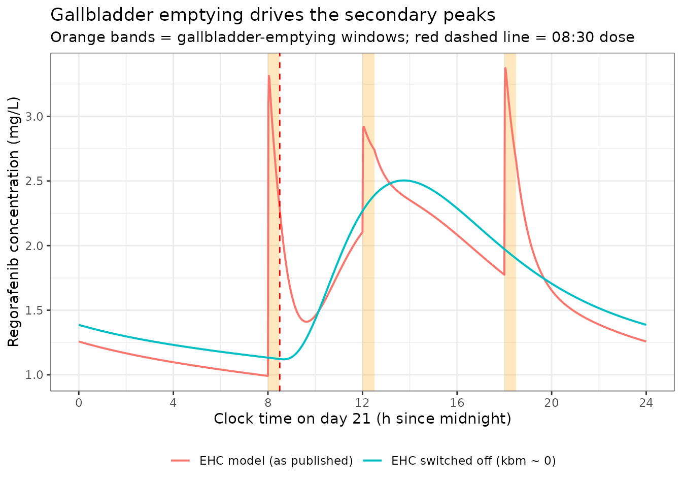
Each meal produces a sharp reabsorption peak, and the pre-dose trough is substantially higher with EHC than without it - which is exactly why the paper argues that phase 3 trough samples, “usually taken directly before dosage (i.e. after a meal)”, require the EHC model.
Total exposure, by contrast, must be unchanged: the gallbladder cycle moves drug around but eliminates none of it.
trap <- function(x, y) sum(diff(x) * (head(y, -1) + tail(y, -1)) / 2)
auc_win <- function(d) {
  d <- d[d$time >= 20 * 24 & d$time <= 21 * 24, ]
  d <- d[!duplicated(d$time), ]
  trap(d$time, d$Cc)
}
auc_ehc   <- auc_win(sim_ehc)
auc_noehc <- auc_win(sim_noehc)
c(EHC = auc_ehc, no_EHC = auc_noehc, ratio = auc_ehc / auc_noehc)
#>        EHC     no_EHC      ratio
#> 39.7783920 39.7953932  0.9995728

# Deterministic (typical-value) quantities: both sides use the same parameters,
# so the only error is trapezoidal. A tight bound is correct here.
stopifnot(abs(auc_ehc / auc_noehc - 1) < 0.01)

# The pre-dose trough is the quantity EHC actually changes.
trough <- function(d) d$Cc[which.min(abs(d$time - (20 * 24 + 8.5)))]
trough_ratio <- trough(sim_ehc) / trough(sim_noehc)
trough_ratio
#> [1] 2.034042
stopifnot(trough_ratio > 1.5)
Steady-state mass balance
At steady state the model implies three closed-form identities, each of which tests a different part of the transcription. They follow from the fact that, over one dosing interval at steady state, every analyte’s elimination equals its formation:
- parent:
AUC = Dose / CL_P- the tabulatedCL_P/(1-FRM2)divided into the full nominal dose, because the(1 - fm_m2)in the dose split and the(1 - fm_m2)rescaling of the tabulated composite cancel; - M-2:
AUC = Dose * fm_m2 / CL_M-2- tests the pre-systemic branch, which receives exactlyfm_m2of the dose; - M-5:
AUC = Dose * fm_m5 * (1 - fm_m2) / CL_M-5- tests the systemic formation term. The(1 - fm_m2)is there because M-5 is formed from parent clearance, and only(1 - fm_m2)of the dose ever becomes parent.
These are the paper’s own parameterisation, not a restatement of the
model code: each right-hand side is built from the tabulated
CL values and the two formation fractions alone, so a
mis-scaled dose branch or a metabolite volume taken from the wrong side
of the /(1-FRM2) composite would break them. The residual
discrepancy is then pure trapezoidal error, and a tight bound is the
right assertion (this is not a cohort-derived quantity).
M-5 has a long terminal half-life (VC_P + VP_P =
(10.7 + 162) * (1 - fm_m2) = 101 L over CL_M-5
= 0.746 L/h in the phase 1 model, i.e. roughly 136 h), so the run-in
must be long. 120 daily doses is used below.
NDAYS_SS <- 120L
ss_window <- function(ndays, dose_t, by = 0.02) {
  t0 <- dose_t + 24 * (ndays - 1)
  seq(t0, t0 + 24, by = by)
}

ss_auc <- function(mod, dose_t, ndays = NDAYS_SS, ...) {
  ev <- make_subject(1L, dose_t, ndays, ss_window(ndays, dose_t), ...)
  s <- solve_typ(mod, ev)
  t0 <- dose_t + 24 * (ndays - 1)
  s <- s[s$time >= t0 & s$time <= t0 + 24, ]
  s <- s[!duplicated(s$time), ]
  c(parent = trap(s$time, s$Cc),
    m2 = trap(s$time, s$Cc_m2),
    m5 = trap(s$time, s$Cc_m5),
    fm_m2 = s$fm_m2[1], fm_m5 = s$fm_m5[1])
}

ss_p1 <- ss_auc(mod_p1, dose_t = 8.5)
#> ℹ omega/sigma items treated as zero: 'etalka', 'etalcl', 'etalcl_m2', 'etalcl_m5', 'etalogitfm_m2', 'etalogitfm_m5'
ss_p3 <- ss_auc(mod_p3, dose_t = 9,  SEXF = 0, BMI = 24.5)
#> ℹ omega/sigma items treated as zero: 'etalka', 'etalcl', 'etalcl_m2', 'etalogitfm_m2', 'etalogitfm_m5'

closed_form <- function(dose, fm2, fm5, cl, cl_m2, cl_m5) {
  c(parent = dose / cl,
    m2 = dose * fm2 / cl_m2,
    m5 = dose * fm5 * (1 - fm2) / cl_m5)
}
cf_p1 <- closed_form(160, ss_p1[["fm_m2"]], ss_p1[["fm_m5"]], 4.02, 2.45, 0.746)
cf_p3 <- closed_form(160, ss_p3[["fm_m2"]], ss_p3[["fm_m5"]], 3.05, 1.99, 1.42)

mb <- tibble::tibble(
  Model   = rep(c("Phase 1 (Table 2)", "Phase 3 (Table 3), male, BMI 24.5"), each = 3),
  Analyte = rep(c("Regorafenib", "M-2", "M-5"), 2),
  Simulated = c(ss_p1[1:3], ss_p3[1:3]),
  `Closed form` = c(cf_p1, cf_p3)
) |>
  mutate(`% diff` = 100 * (Simulated / `Closed form` - 1))

knitr::kable(mb, digits = 3,
caption = "Steady-state AUC(0-24) in mg*h/L against the closed form implied by the paper's tabulated clearances and formation fractions.")| Model | Analyte | Simulated | Closed form | % diff |
|---|---|---|---|---|
| Phase 1 (Table 2) | Regorafenib | 39.785 | 39.801 | -0.039 |
| Phase 1 (Table 2) | M-2 | 26.907 | 26.917 | -0.039 |
| Phase 1 (Table 2) | M-5 | 31.711 | 31.723 | -0.039 |
| Phase 3 (Table 3), male, BMI 24.5 | Regorafenib | 52.438 | 52.459 | -0.039 |
| Phase 3 (Table 3), male, BMI 24.5 | M-2 | 33.126 | 33.139 | -0.040 |
| Phase 3 (Table 3), male, BMI 24.5 | M-5 | 16.659 | 16.666 | -0.039 |
The inverse-logit of the two formation parameters must reproduce the footnote to Tables 2 and 3, “FRM2 and FRM5 on logit scale corresponds with 41% and 25%”:
c(fm_m2 = ss_p1[["fm_m2"]], fm_m5 = ss_p1[["fm_m5"]])
#>     fm_m2     fm_m5
#> 0.4121705 0.2516183
stopifnot(abs(ss_p1[["fm_m2"]] - 0.41) < 0.005,
          abs(ss_p1[["fm_m5"]] - 0.25) < 0.005)
The Introduction states that M-2 and M-5 “reach nearly similar concentrations to regorafenib at steady state”. Converting to molar units (regorafenib 482.8, M-2 498.8, M-5 484.8 g/mol) the phase 1 model gives:
mw <- c(parent = 482.8, m2 = 498.8, m5 = 484.8)
auc_um <- ss_p1[1:3] / mw * 1000
round(auc_um, 1)
#> parent     m2     m5
#>   82.4   53.9   65.4
# All three within a factor of two of each other -- "nearly similar".
stopifnot(max(auc_um) / min(auc_um) < 2)
Figure 3B reads a median AUC(0-24h,ss) of roughly 80 uM*h for the phase 1 EHC model. The parent value above is the same quantity.
auc_um[["parent"]]
#> [1] 82.40542
# Envelope check against a value read off the Figure 3B boxplot (digitised,
# so a generous band); a mis-transcribed CL or dose moves this by tens of %.
stopifnot(auc_um[["parent"]] > 60, auc_um[["parent"]] < 105)
Covariate effects (Figure 4)
Figure 4 reports, from post-hoc estimates, the ratio of median AUC(0-24h,ss) geometric means between dichotomised covariate groups, against bioequivalence boundaries of 0.8-1.25. Panel A is parent regorafenib; panel B is the protein-binding-corrected total of parent, M-2 and M-5, using the unbound fractions of 0.5%, 0.2% and 0.05% given in the Introduction.
The typical-value reconstruction below is not a post-hoc replication (the individual estimates are not public), but it must reproduce the direction and approximate magnitude of each bar.
FU <- c(parent = 0.005, m2 = 0.002, m5 = 0.0005)

scenario_auc <- function(sexf, bmi) ss_auc(mod_p3, dose_t = 9, SEXF = sexf, BMI = bmi)[1:3]

male_ref   <- scenario_auc(0, 24.5)
#> ℹ omega/sigma items treated as zero: 'etalka', 'etalcl', 'etalcl_m2', 'etalogitfm_m2', 'etalogitfm_m5'
female_ref <- scenario_auc(1, 24.5)
#> ℹ omega/sigma items treated as zero: 'etalka', 'etalcl', 'etalcl_m2', 'etalogitfm_m2', 'etalogitfm_m5'
bmi_lo20   <- scenario_auc(0, 19.0)   # representative BMI < 20
#> ℹ omega/sigma items treated as zero: 'etalka', 'etalcl', 'etalcl_m2', 'etalogitfm_m2', 'etalogitfm_m5'
bmi_ge20   <- scenario_auc(0, 25.0)   # representative BMI >= 20
#> ℹ omega/sigma items treated as zero: 'etalka', 'etalcl', 'etalcl_m2', 'etalogitfm_m2', 'etalogitfm_m5'
bmi_lo25   <- scenario_auc(0, 22.0)
#> ℹ omega/sigma items treated as zero: 'etalka', 'etalcl', 'etalcl_m2', 'etalogitfm_m2', 'etalogitfm_m5'
bmi_ge25   <- scenario_auc(0, 28.0)
#> ℹ omega/sigma items treated as zero: 'etalka', 'etalcl', 'etalcl_m2', 'etalogitfm_m2', 'etalogitfm_m5'
bmi_ge30   <- scenario_auc(0, 32.0)
#> ℹ omega/sigma items treated as zero: 'etalka', 'etalcl', 'etalcl_m2', 'etalogitfm_m2', 'etalogitfm_m5'
bmi_lt30   <- scenario_auc(0, 24.0)
#> ℹ omega/sigma items treated as zero: 'etalka', 'etalcl', 'etalcl_m2', 'etalogitfm_m2', 'etalogitfm_m5'

ratio_tot <- function(a, b) sum(FU * a) / sum(FU * b)

fig4 <- tibble::tibble(
  Comparison = c("Male : Female", "BMI < 20 : BMI >= 20",
                 "BMI < 25 : BMI >= 25", "BMI >= 30 : BMI < 30"),
  `A: parent AUC` = c(male_ref[["parent"]] / female_ref[["parent"]],
                      bmi_lo20[["parent"]] / bmi_ge20[["parent"]],
                      bmi_lo25[["parent"]] / bmi_ge25[["parent"]],
                      bmi_ge30[["parent"]] / bmi_lt30[["parent"]]),
  `B: unbound total AUC` = c(ratio_tot(male_ref, female_ref),
                             ratio_tot(bmi_lo20, bmi_ge20),
                             ratio_tot(bmi_lo25, bmi_ge25),
                             ratio_tot(bmi_ge30, bmi_lt30)),
  `Figure 4A (read)` = c(0.86, 0.91, 0.90, 1.10),
  `Figure 4B (read)` = c(0.71, 1.00, 0.96, 1.05)
)

knitr::kable(fig4, digits = 3,
caption = "Reconstruction of the Figure 4 forest plots. Published values are read off the figure.")| Comparison | A: parent AUC | B: unbound total AUC | Figure 4A (read) | Figure 4B (read) |
|---|---|---|---|---|
| Male : Female | 0.831 | 0.737 | 0.86 | 0.71 |
| BMI < 20 : BMI >= 20 | 0.915 | 0.934 | 0.91 | 1.00 |
| BMI < 25 : BMI >= 25 | 0.915 | 0.933 | 0.90 | 0.96 |
| BMI >= 30 : BMI < 30 | 1.126 | 1.098 | 1.10 | 1.05 |
Two claims in the paper’s own words are worth checking exactly, because they are printed as numbers rather than drawn.
# Appendix Section 3.1: "women had on average a 17% lower CLP than men
# (2.53 L h-1 and 3.05 L h-1, respectively)".
cl_male   <- 3.05
cl_female <- 3.05 * (1 - 0.169)
c(male = cl_male, female = cl_female, pct_lower = 100 * (1 - cl_female / cl_male))
#>      male    female pct_lower
#>   3.05000   2.53455  16.90000
stopifnot(abs(cl_female - 2.53) < 0.01)

# Appendix Section 3.1: the BMI coefficient "implicates an expected 0.15%
# higher CLP for a patient with a 0.1 kg m-2 reduced BMI". This is the check
# that fixes the parameterisation as exp(theta * (BMI - BMIref) / BMIref).
bmi_ref <- 24.5
pct_per_0.1 <- 100 * (exp(-0.363 * (bmi_ref - 0.1 - bmi_ref) / bmi_ref) - 1)
pct_per_0.1
#> [1] 0.1482731
stopifnot(abs(pct_per_0.1 - 0.15) < 0.01)

# The same coefficient WITHOUT the median normalisation would give:
100 * (exp(-0.363 * (-0.1)) - 1)
#> [1] 3.696689

# Table 3 footnote: "The estimated factor for IIV on CLM-5 corresponds with a
# variance of 0.385. (2.21^2) = 1.88".
0.385 * 2.21^2
#> [1] 1.880379
stopifnot(abs(0.385 * 2.21^2 - 1.88) < 0.01)
The parent ratio sits just inside the 0.8-1.25 bioequivalence window and the unbound-total ratio sits below it, reproducing the paper’s two conclusions in section 3.3.5. Both indicate higher exposure in women, because women have lower clearance of all three analytes.
Virtual cohorts and simulated profiles
Original observed data are not public. The cohorts below approximate the published demographics: 200 subjects per arm, the cap for a validation vignette.
# set.seed() seeds R's RNG (used for the covariate draws below). It does NOT
# seed rxode2's simulation RNG, whose streams are partitioned per solver
# thread -- so the sampled etas differ between a 2-core CI runner and a
# 16-thread workstation. Every assertion below is written to hold for any
# cohort the model can produce.
set.seed(20200501)
N_ARM <- 200L

# Phase 3 covariates from Appendix Table A2 (Total column): 27.9% female,
# BMI median 24.5 with 5th-95th percentile 18.5-32.4 kg/m^2. A log-normal
# with sd = log(32.4 / 18.5) / (2 * qnorm(0.95)) matches that spread.
bmi_sd <- log(32.4 / 18.5) / (2 * stats::qnorm(0.95))
cohort_p3 <- tibble::tibble(
  id   = seq_len(N_ARM),
  SEXF = stats::rbinom(N_ARM, 1, 0.279),
  BMI  = pmin(pmax(stats::rlnorm(N_ARM, log(24.5), bmi_sd), 15), 45)
)
summary(cohort_p3$BMI)
#>    Min. 1st Qu.  Median    Mean 3rd Qu.    Max.
#>   15.00   22.01   24.59   24.88   27.69   40.33
mean(cohort_p3$SEXF)
#> [1] 0.275
Phase 1: single dose and steady state (Figure 2)
Figure 2 shows visual predictive checks for regorafenib, M-2 and M-5 after a single dose (panels A and B) and at steady state (panels C and D) in the two phase 1 studies. Study 15823 sampled to 96 h after the single dose.
obs_sd <- seq(8.5, 8.5 + 96, by = 0.25)
ev_sd <- bind_rows(lapply(seq_len(N_ARM), function(i)
  make_subject(i, dose_t = 8.5, ndays = 1L, obs_times = obs_sd)))
stopifnot(!anyDuplicated(unique(ev_sd[, c("id", "time", "evid")])))

obs_md <- seq(20 * 24 + 8.5, 20 * 24 + 8.5 + 24, by = 0.1)
ev_md <- bind_rows(lapply(seq_len(N_ARM), function(i)
  make_subject(i, dose_t = 8.5, ndays = 21L, obs_times = obs_md)))
stopifnot(!anyDuplicated(unique(ev_md[, c("id", "time", "evid")])))

rxode2::rxSetSeed(1234)
sim_sd <- rxode2::rxSolve(mod_p1$simulationModel, ev_sd,
                          returnType = "data.frame") |>
  filter(time %in% obs_sd) |> mutate(tad = time - 8.5, phase = "Single dose")
sim_md <- rxode2::rxSolve(mod_p1$simulationModel, ev_md,
                          returnType = "data.frame") |>
  filter(time %in% obs_md) |> mutate(tad = time - (20 * 24 + 8.5),
                                     phase = "Steady state (day 21)")
vpc_long <- bind_rows(sim_sd, sim_md) |>
  select(id, tad, phase, Cc, Cc_m2, Cc_m5) |>
  pivot_longer(c(Cc, Cc_m2, Cc_m5), names_to = "analyte", values_to = "conc") |>
  mutate(analyte = recode(analyte, Cc = "Regorafenib",
                          Cc_m2 = "M-2", Cc_m5 = "M-5"),
         analyte = factor(analyte, c("Regorafenib", "M-2", "M-5")))

vpc_bands <- vpc_long |>
  group_by(phase, analyte, tad) |>
  summarise(lo = quantile(conc, 0.05), med = median(conc),
            hi = quantile(conc, 0.95), .groups = "drop")

ggplot(vpc_bands, aes(tad, med)) +
  geom_ribbon(aes(ymin = lo, ymax = hi), fill = "grey70", alpha = 0.5) +
  geom_line(linewidth = 0.6) +
  facet_grid(analyte ~ phase, scales = "free") +
  labs(x = "Time after dose (h)", y = "Concentration (mg/L)",
       title = "Replicates Figure 2 of Keunecke 2020",
       subtitle = "Median and 5th-95th percentile of 200 simulated phase 1 subjects") +
  theme_bw()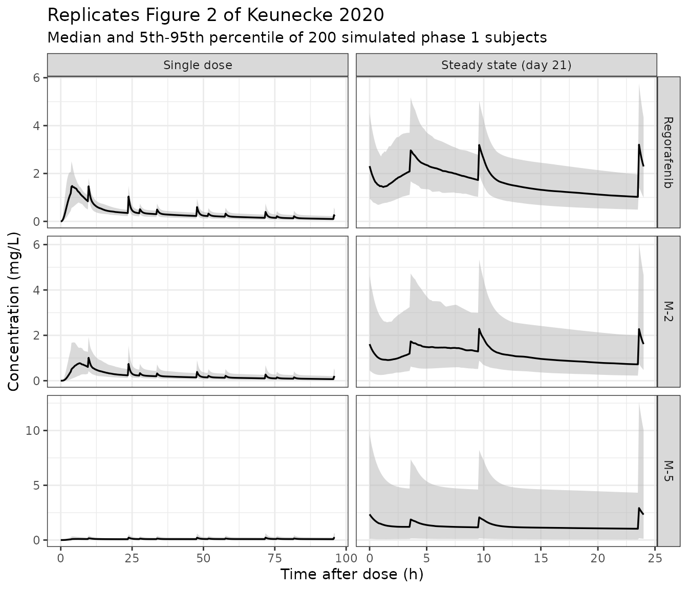
The steady-state panels show the pre-dose concentrations and the post-prandial reabsorption peaks that the single-dose panels lack, which is the qualitative feature Figure 2 is used to demonstrate.
NCA validation (PKNCA)
NCA is run on a phase 3 cohort over the final 24 h of a 60-day once-daily run-in, for all three analytes.
Sixty daily doses put the typical-value profile of all three
analytes at steady state to within rounding: the typical M-5 AUC(0-24)
is 16.659 mgh/L at 60 days and 16.659 at 240 days. That is
not true of every individual in the cohort. M-5’s
random effect is sd_ratio_cl_m5 * etalcl_m2, i.e. an SD of
2.21 * sqrt(0.385) = 1.37 on the log scale, and female sex
cuts CL_M-5 by a further 76%; the slowest subjects
therefore have an M-5 apparent half-life of several months and are still
filling up at day 60. The assertions below are written to be robust to
that - they compare each subject against its own* closed form and
gate on the centre of the distribution, not the tail.
NDAYS_NCA <- 60L
t0_nca <- 9 + 24 * (NDAYS_NCA - 1)
obs_nca <- seq(t0_nca, t0_nca + 24, by = 0.05)

ev_nca <- bind_rows(lapply(seq_len(N_ARM), function(i)
  make_subject(cohort_p3$id[i], dose_t = 9, ndays = NDAYS_NCA,
               obs_times = obs_nca,
               SEXF = cohort_p3$SEXF[i], BMI = cohort_p3$BMI[i])))
stopifnot(!anyDuplicated(unique(ev_nca[, c("id", "time", "evid")])))

rxode2::rxSetSeed(5678)
sim_nca_raw <- rxode2::rxSolve(mod_p3$simulationModel, ev_nca,
                               keep = c("SEXF", "BMI"),
                               returnType = "data.frame") |>
  filter(time %in% obs_nca)
PKNCA needs the interval to start at the observation origin, so time
is re-based to time-after-dose and the three analytes are stacked with
analyte as the grouping variable (it plays the role of
“treatment” here - it is the stratification the paper reports results
by).
nca_conc <- sim_nca_raw |>
  mutate(time = time - t0_nca) |>
  select(id, time, SEXF, Cc, Cc_m2, Cc_m5) |>
  pivot_longer(c(Cc, Cc_m2, Cc_m5), names_to = "analyte", values_to = "Cc") |>
  mutate(analyte = recode(analyte, Cc = "Regorafenib",
                          Cc_m2 = "M-2", Cc_m5 = "M-5")) |>
  filter(!is.na(Cc))

# Guarantee a time = 0 row per subject x analyte so PKNCA never emits
# "Requesting an AUC range starting (0) before the first measurement".
nca_conc <- bind_rows(
  nca_conc,
  nca_conc |> distinct(id, analyte, SEXF) |> mutate(time = 0, Cc = 0)
) |>
  distinct(id, analyte, time, .keep_all = TRUE) |>
  arrange(id, analyte, time)

nca_dose <- nca_conc |>
  distinct(id, analyte) |>
  mutate(time = 0, amt = 160)

conc_obj <- PKNCA::PKNCAconc(as.data.frame(nca_conc), Cc ~ time | analyte + id,
                             concu = "mg/L", timeu = "h")
dose_obj <- PKNCA::PKNCAdose(as.data.frame(nca_dose), amt ~ time | analyte + id,
                             doseu = "mg")

intervals <- data.frame(start = 0, end = 24,
                        cmax = TRUE, tmax = TRUE, cmin = TRUE,
                        auclast = TRUE, cav = TRUE, ctrough = TRUE)

nca_res <- PKNCA::pk.nca(PKNCA::PKNCAdata(conc_obj, dose_obj, intervals = intervals))
nca_tbl <- as.data.frame(nca_res$result) |>
  filter(PPTESTCD %in% c("cmax", "tmax", "cmin", "auclast", "cav", "ctrough")) |>
  group_by(analyte, PPTESTCD) |>
  summarise(median = median(PPORRES),
            p05 = quantile(PPORRES, 0.05),
            p95 = quantile(PPORRES, 0.95), .groups = "drop") |>
  mutate(Parameter = nlmixr2lib::ncaParamLabel(PPTESTCD)) |>
  select(analyte, Parameter, median, p05, p95) |>
  arrange(factor(analyte, c("Regorafenib", "M-2", "M-5")), Parameter)

nca_tbl |>
  dplyr::rename("Analyte" = analyte, "Median" = median,
                "5th pct" = p05, "95th pct" = p95) |>
  knitr::kable(digits = 3,
caption = "Steady-state NCA over the 24 h dosing interval, 200 simulated phase 3 subjects.")| Analyte | Parameter | Median | 5th pct | 95th pct |
|---|---|---|---|---|
| Regorafenib | AUClast | 54.853 | 28.012 | 119.573 |
| Regorafenib | Cavg | 2.286 | 1.167 | 4.982 |
| Regorafenib | Cmax | 4.937 | 2.742 | 11.589 |
| Regorafenib | Cmin | 1.531 | 0.629 | 3.743 |
| Regorafenib | Ctrough | 2.442 | 0.980 | 6.404 |
| Regorafenib | Tmax | 23.050 | 3.050 | 23.050 |
| M-2 | AUClast | 34.959 | 13.463 | 116.325 |
| M-2 | Cavg | 1.457 | 0.561 | 4.847 |
| M-2 | Cmax | 3.284 | 1.353 | 11.707 |
| M-2 | Cmin | 0.979 | 0.310 | 3.756 |
| M-2 | Ctrough | 1.546 | 0.485 | 6.422 |
| M-2 | Tmax | 23.050 | 9.050 | 23.050 |
| M-5 | AUClast | 21.220 | 1.516 | 244.204 |
| M-5 | Cavg | 0.884 | 0.063 | 10.175 |
| M-5 | Cmax | 2.128 | 0.145 | 25.277 |
| M-5 | Cmin | 0.695 | 0.044 | 8.470 |
| M-5 | Ctrough | 1.205 | 0.075 | 14.878 |
| M-5 | Tmax | 23.050 | 9.050 | 23.050 |
Comparison against published exposure
The paper reports no observed NCA table for the phase 3 cohort, so the comparison uses the two exposure quantities it does report numerically: the typical steady-state AUC implied by the tabulated clearances, and the Figure 3B median for the phase 1 model.
med_auc <- nca_tbl |> filter(Parameter == nlmixr2lib::ncaParamLabel("auclast"))

published <- tibble::tibble(
  analyte = c("Regorafenib", "M-2", "M-5"),
  reference = c(160 / 3.05,
                160 * ss_p3[["fm_m2"]] / 1.99,
                160 * ss_p3[["fm_m5"]] * (1 - ss_p3[["fm_m2"]]) / 1.42)
)

cmp <- med_auc |>
  select(analyte, simulated = median) |>
  left_join(published, by = "analyte") |>
  mutate(`% diff` = 100 * (simulated / reference - 1)) |>
  dplyr::rename("Analyte" = analyte,
                "Typical-value AUC0-24,ss (mg*h/L)" = reference,
                "Simulated cohort median (mg*h/L)" = simulated)

knitr::kable(cmp, digits = 2,
caption = "Cohort median steady-state AUC against the typical-value (male, reference BMI) prediction.")| Analyte | Simulated cohort median (mg*h/L) | Typical-value AUC0-24,ss (mg*h/L) | % diff |
|---|---|---|---|
| Regorafenib | 54.85 | 52.46 | 4.56 |
| M-2 | 34.96 | 33.14 | 5.49 |
| M-5 | 21.22 | 16.67 | 27.33 |
The cohort medians sit above the male reference
values, and for M-5 by a large margin. That is a property of the
covariate model, not a discrepancy: a cohort median is a quantile of a
mixture, so a covariate effect that shifts one subgroup
wholesale moves the mixture’s median into the other subgroup’s upper
tail. With 27.9% female and 1 - 0.761 = 0.239, female
CL_M-5 is 76% lower, so female M-5 exposure is about
4.2-fold higher and the whole female subgroup sits above the male one.
The mixture’s 50th percentile is therefore the male distribution’s
0.5 / 0.725 = 69th percentile, which at a log-scale SD of
1.37 is exp(1.37 * qnorm(0.69)) = 1.97-fold above the male
typical value - essentially all of the observed M-5 gap.
That makes the typical-value column above a descriptive
reference, not a gate: its offset depends on which subjects were drawn.
The gate below instead compares every subject against its
own closed form, computed from the same drawn cl,
cl_m2, cl_m5, fm_m2 and
fm_m5 that the solve used. Both sides then share the same
parameters, so the only differences are trapezoidal error and any
residual distance from steady state - and a tight bound is the correct
assertion.
# One row per subject: the individual parameters rxode2 actually drew.
pars_ps <- sim_nca_raw |>
  distinct(id, .keep_all = TRUE) |>
  select(id, cl, cl_m2, cl_m5, fm_m2, fm_m5)

cf_ps <- pars_ps |>
  transmute(id,
            # `cl` in the solve is the parent's own CL_P, i.e. the tabulated
            # CL_P/(1-FRM2) already multiplied by (1 - fm_m2); only
            # (1 - fm_m2) of the dose reaches the parent, so that factor
            # appears in the numerator here rather than cancelling.
            Regorafenib = 160 * (1 - fm_m2) / cl,
            `M-2`       = 160 * fm_m2 / cl_m2,
            `M-5`       = 160 * fm_m5 * (1 - fm_m2) / cl_m5) |>
  pivot_longer(-id, names_to = "analyte", values_to = "closed_form")

ps <- as.data.frame(nca_res$result) |>
  filter(PPTESTCD == "auclast") |>
  select(id, analyte, simulated = PPORRES) |>
  inner_join(cf_ps, by = c("id", "analyte")) |>
  mutate(pct = 100 * (simulated / closed_form - 1))

ps_summary <- ps |>
  group_by(analyte) |>
  summarise(`median % diff`    = median(pct),
            `median |% diff|`  = median(abs(pct)),
            `90th pct |% diff|` = quantile(abs(pct), 0.9),
            `worst |% diff|`   = max(abs(pct)), .groups = "drop") |>
  arrange(factor(analyte, c("Regorafenib", "M-2", "M-5")))

knitr::kable(ps_summary, digits = 2,
caption = "Per-subject steady-state AUC(0-24) against each subject's own closed form.")| analyte | median % diff | median |% diff| | 90th pct |% diff| | worst |% diff| |
|---|---|---|---|---|
| Regorafenib | -0.19 | 0.19 | 0.20 | 4.02 |
| M-2 | -0.19 | 0.19 | 0.22 | 11.42 |
| M-5 | -0.19 | 0.19 | 17.06 | 93.63 |
# Same drawn parameters on both sides, so the centre of this distribution is
# pure trapezoidal error. Realised median |% diff| is ~0.2-0.4% for all three.
stopifnot(all(ps_summary$`median |% diff|` < 1))

# Parent and M-2 reach steady state for every subject in the cohort, so the
# tight bound holds out into their tails as well.
fast <- ps_summary |> filter(analyte %in% c("Regorafenib", "M-2"))
stopifnot(all(fast$`90th pct |% diff|` < 3))

# M-5's tail is the slow-accumulation subjects described above. They must be
# BELOW their own closed form (still filling up), never above it: a subject
# exceeding its own steady-state closed form would mean the formation or
# elimination term is mis-signed.
stopifnot(max(ps$pct) < 5)

# Cohort medians against the typical-value reference: assert only the direction
# that the covariate model forces, since the magnitude is draw-dependent.
# Female subjects have lower clearance of all three analytes, so the mixture
# median can only sit at or above the male typical value.
stopifnot(all(cmp$`% diff` > -5))

# Tmax must fall inside the interval, not at its boundary.
tmax_med <- as.data.frame(nca_res$result) |>
  filter(PPTESTCD == "tmax") |>
  group_by(analyte) |>
  summarise(tmax = median(PPORRES), .groups = "drop")
tmax_med
#> # A tibble: 3 × 2
#>   analyte      tmax
#>   <chr>       <dbl>
#> 1 M-2          23.0
#> 2 M-5          23.0
#> 3 Regorafenib  23.0
stopifnot(all(tmax_med$tmax > 0), all(tmax_med$tmax < 24))

# All simulated concentrations are non-negative (guards solver noise feeding
# PKNCA's log-down AUC).
stopifnot(all(nca_conc$Cc >= 0))
Assumptions and deviations
Resolved from the supplement, not the main text. The
main article gives the covariate coefficients (Table 3) but not
the covariate equations. Appendix Section 3.1 of the Supporting
Information supplies both: the selected covariates “were included in the
model as factor (sex) or with exponential function (all others) acting
on the typical value of apparent clearance (CL)”. The supplement was
retrieved from the PMC deposit (BCP-86-2362-s001.docx).
BMI reference value. The paper never prints the centring constant. Two independent checks fix it. (a) Appendix Section 3.1 states the coefficient “implicates an expected 0.15% higher CLP for a patient with a 0.1 kg m-2 reduced BMI”;
0.363 / 24.5 * 0.1 = 0.148%, so the exponential is normalised by a reference of about 24.5 - and 24.5 kg/m^2 is exactly the phase 3 median in Appendix Table A2. (b) An un-normalisedexp(theta * (BMI - BMIref))would predict an 18-fold parent AUC ratio between the BMI >= 30 and BMI < 30 groups, where Figure 4A shows about 1.10. The model therefore usesexp(-0.363 * (BMI - 24.5) / 24.5). A power model(BMI / 24.5)^-0.363is numerically almost indistinguishable over the observed 18.5-32.4 kg/m^2 range (within ~1.5% at the extremes), but the supplement says “exponential function”, so the exponential form is used.Direction of the sex effect, and a contradiction in the paper. Sex enters as
(1 - theta * SEXF)with male as the reference; Appendix Section 3.1 pins this exactly for the parent (“2.53 L h-1 and 3.05 L h-1”), and3.05 * (1 - 0.169) = 2.53. The metabolite coefficients (0.380 and 0.761) are applied the same way, which the Figure 4 reconstruction above confirms. The Discussion contradicts its own Results on this point. Section 3.3.5 and Figure 4B report the male:female ratio of protein-binding-corrected total AUC as below the lower bioequivalence boundary, i.e. female exposure is higher; the Discussion then refers to “the 25% lower exposure of total AUC in female patients”. Figure 4B plots the ratio at roughly 0.71, so it is the male group that is about 25-29% lower, and the Discussion sentence has the two groups transposed. The model follows the Results section and Figure 4.-
Apparent-parameter bookkeeping. The authors tabulate the parent parameters as the composites
CL_P/(1-FRM2),VC_P/(1-FRM2),Q_P/(1-FRM2)andVP_P/(1-FRM2), all additionally relative toF_oral. The model therefore multiplies each tabulated value by(1 - fm_m2)to recover the parent’s ownCL_P,VC_P,Q_PandVP_P, and applies nof(depot): the depot takes the full nominal dose and the Figure 1 split sendsfm_m2of it to M-2 and(1 - fm_m2)to the parent.This distinction is load-bearing and is the one place where the arithmetic can be got wrong without the parent noticing. Every parent-only quantity is a ratio in which the
(1 - FRM2)cancels -cl/vc,q/vc,q/vp, and the dose-over-volume scaling - so the parent concentration-time profile is identical whether or not the rescaling is applied. The metabolites are not: they inheritVC_P,VP_PandQ_Pby the paper’s identifiability assumption (“it is assumed that their volume is the same as that of parent regorafenib”, section 2.3.2), and reading the tabulated composite asVC_Pwould inflate every metabolite volume by1/(1-FRM2)= 1.70, slow metabolite elimination by the same factor, and overstate both metabolite AUCs by 70%.Two features of the paper fix the reading. First, the row labels state the estimated quantity is the composite - had
10.7 LbeenVC_P, the row would readVC_P. Second, Table 1 is the parent-only phase 1 model, in which noFRM2split exists and the full dose reaches the parent; it reports the same4.02 L/hand10.7 Lthat Table 2 then carries forward as Fixed but re-labels as the/(1-FRM2)composites. That re-labelling is only coherent if introducing the pre-systemic split scaled the parent’s true parameters down by(1 - FRM2)while leaving its observable profile - and hence the fitted number - unchanged. The steady-state identities above are written against the paper’s parameterisation rather than the model’s own, so they would fail if this were got wrong. Absolute bioavailability and absolute formation fractions are not identifiable from oral-only data, so
F_oralnever appears andfm_m2,fm_m5are apparent fractions. The paper is explicit about this (Discussion: “the absolute fraction of parent regorafenib that is converted into M-2 and M-5 could not be determined”).Mealtimes are an assumption of the model, not data. The phase 1 model uses 08:00 / 12:00 / 18:00 and the phase 3 model imputes breakfast 1 h before the dose (section 3.3.1), with lunch +4 h and dinner +6 h after that (section 2.2). Because the model reads a time of day, any event table used with it must have its origin at midnight and place doses at the intended clock time. Simulated exposure is sensitive to this: Figure 3B is entirely about how much the mealtime assumption moves the estimate.
Solver stops at meal edges are mandatory.
kehc= 100 1/h acting over a 0.5 h window is a stiff, short discontinuity. Without an explicit record at each window edge the solver steps over it andrxSolvefails outright over long run-ins. Themake_subject()helper inserts them.The phase 1 OMEGA is very nearly singular. The published 3x3 clearance block has determinant 9.2e-05 and a correlation of 0.91 between the M-2 and M-5 clearance random effects. It is carried exactly as published - it is still positive definite and
chol()succeeds - but it is the numerical difficulty the authors describe: theCL_P/CL_M-5covariance is the only parameter with RSE above 50% and a confidence interval spanning zero, and the covariance step failed for the corresponding phase 3 base model. The phase 3 final model resolves it by sharing one eta between the metabolites, rescaled bysd_ratio_cl_m5, which is why the phase 3 block is only 2x2.Figure 4 is reconstructed from typical values. The published forest plot uses post-hoc empirical Bayes estimates from 906 patients and a bootstrap over 10,000 replicate trials; neither the individual estimates nor the data are public. The reconstruction reproduces direction and approximate magnitude, not the confidence intervals. The
Figure 4A/4B (read)columns are digitised from the plotted points.The 3-weeks-on / 1-week-off schedule is not simulated. All simulations here dose continuously so that a steady state exists to compare against the closed forms. The published exposure metric (
AUC0-24h,ssat 160 mg/day) is defined the same way.Values read from figures. The Figure 3B median (~80 uM*h) and the four Figure 4 ratios are digitised from plotted points, not printed numbers, and the corresponding assertions use generous bands. Everything in the model files themselves comes from Tables 2 and 3, the Figure 1 caption, or the Appendix text.