Eptinezumab (Baker 2020) • nlmixr2lib

library(nlmixr2lib)
library(rxode2)
#> rxode2 5.1.8 using 2 threads (see ?getRxThreads)
#>   no cache: create with `rxCreateCache()`
library(dplyr)
#> 
#> Attaching package: 'dplyr'
#> The following objects are masked from 'package:stats':
#> 
#>     filter, lag
#> The following objects are masked from 'package:base':
#> 
#>     intersect, setdiff, setequal, union
library(tidyr)
library(ggplot2)
library(PKNCA)
#> 
#> Attaching package: 'PKNCA'
#> The following object is masked from 'package:stats':
#> 
#>     filter

Eptinezumab population PK model

Eptinezumab is a humanized IgG1 monoclonal antibody that binds both the alpha and beta forms of calcitonin gene-related peptide (CGRP). It is given as an intravenous infusion every 12 weeks for the prevention of episodic and chronic migraine. Baker et al. (2020) pooled eight studies (2123 healthy participants and patients, IV doses 1-1000 mg) and described the free-eptinezumab plasma concentrations with a two-compartment model with linear elimination, fitted in Phoenix NLME 8.0 (FOCE-ELS).

The journal article reports the typical clearance (0.00620 L/h) and central volume (3.64 L), the between-subject variability on both, the additive residual error, the alpha and beta half-lives (0.93 and 27 days) and the list of retained covariates, but not the covariate coefficients, the peripheral parameters or the proportional residual error. Those come from the sponsor’s parameter table (report ALD403-088-PK Table 7), which is reproduced as Table 12 of the FDA Clinical Pharmacology Review of BLA 761119 (Vyepti). The EMA assessment report (EMA/9446/2022) Table 6 gives the stepwise covariate build, which shows how many parameters each weight effect used.

Article: Pharmacol Res Perspect 2020;8(2):e00567
FDA review: BLA 761119 Clinical Pharmacology Review
EMA assessment report: Vyepti EPAR

Population

From Baker 2020 section 3.1 and Table 1: 2123 participants from studies CLIN-001, -002, -005, -006, -010, -011, -012 and -013 received eptinezumab. They were mostly female (83.8%), white (88.5%) and ADA-negative at baseline (83.8%), with median age 39.0 years (18-71) and median body weight 74.2 kg (39.2-190). Renal function was normal in 55.3%, mildly decreased in 41.9% and moderately decreased in 2.7%. The FDA review (section 4.3.1) gives the disease split: 83 healthy participants, 727 with episodic migraine (EM) and 1313 with chronic migraine (CM), contributing 15135 quantifiable concentrations. Mean baseline monthly migraine days (MMD) were 16.5 (CLIN-005, CM), 8.7 (CLIN-006, EM) and 16.1 (CLIN-011, CM).

The same information is recorded in the model file’s population metadata.

Source trace

Element	Source location	Value / form
Structure	Baker 2020 section 3.2; FDA review section 4.3.1	2-compartment, IV infusion, linear elimination
CL	Baker 2020 section 3.2; FDA review Table 12	0.00620 L/h
Vc	FDA review Table 12 (Baker 2020 section 3.2: 3.64 L)	3.636 L
Q (CLp)	FDA review Table 12	0.039 L/h
Vp (‘Vd’)	FDA review Table 12 and its footnote	2.012 L
WT on CL and Q	FDA review Table 12; EMA report Table 6 step 1	(WT/70)^0.709, one shared exponent
WT on Vc and Vp	FDA review Table 12; EMA report Table 6 step 2	(WT/70)^0.544, one shared exponent
EM, CM on CL	FDA review Table 12	exp(-0.231), exp(-0.272)
Baseline MMD on CL	FDA review Table 12	(MDBASE/13.0)^0.044
Capped CrCl on CL	FDA review Table 12 and footnote	(min(CrCl, 150)/118)^0.162
EM, CM on Vc	FDA review Table 12	exp(-0.311), exp(-0.422)
Male on Vc	FDA review Table 12	exp(0.091)
BSV CL, Vc	Baker 2020 section 3.2; FDA review Table 12	29.0%, 31.0% CV; omega = log(CV^2 + 1) (Table 12 Note 1)
BSV Q, Vp	FDA review Table 12	111.3%, 34.8% CV
CLp-Vp correlation	EMA report Table 6 footnote a	estimated, value not printed; set to 0
Residual error form	Baker 2020 section 2.2.1 equation	C = f (1 + eps_p) + eps_a
Additive error	Baker 2020 section 3.2; FDA review Table 12	37.5 ng/mL = 0.0375 ug/mL
Proportional error	FDA review Table 12; EMA report	25.2%
Alpha, beta half-life	Baker 2020 section 3.2	0.93 and 27 days (used as a check)
Covariate forest plot	Baker 2020 Figure 4	AUCtau,ss ratios (used as a check)
Single-dose exposure	Baker 2020 Table 2	AUC0-12wk, Cmax, Cavg, Ctrough by dose
Accumulation	Baker 2020 Table 3	Rac(AUC) 1.13-1.15, Rac(Cmax) 1.08-1.10

Typical-value checks

Alpha and beta half-lives

The paper’s half-lives were not used to build the model, so recovering them from the Table 12 disposition parameters is an independent check that Q and Vp were read correctly. This is a closed-form calculation on the reference subject.

mod <- readModelDb("Baker_2020_eptinezumab")
ini_df <- rxode2::rxode2(mod)$iniDf
#> ℹ parameter labels from comments will be replaced by 'label()'
th <- setNames(ini_df$est, ini_df$name)
cl <- exp(th[["lcl"]])
vc <- exp(th[["lvc"]])
q <- exp(th[["lq"]])
vp <- exp(th[["lvp"]])
k10 <- cl / vc
k12 <- q / vc
k21 <- q / vp
s <- k10 + k12 + k21
p <- k10 * k21
lambda <- c((s + sqrt(s^2 - 4 * p)) / 2, (s - sqrt(s^2 - 4 * p)) / 2)
thalf_day <- log(2) / lambda / 24
hl <- data.frame(
  Phase = c("alpha", "beta"),
  Model = signif(thalf_day, 3),
  Published = c(0.93, 27)
)
knitr::kable(hl, caption = "Half-lives (days), reference subject vs Baker 2020 section 3.2.")

Half-lives (days), reference subject vs Baker 2020 section 3.2.
Phase	Model	Published
alpha	0.94	0.93
beta	26.90	27.00

stopifnot(
  abs(thalf_day[1] - 0.93) < 0.02,
  abs(thalf_day[2] - 27) < 0.5
)

Figure 4: covariate effects on steady-state exposure

Figure 4 reports the ratio of steady-state AUC over a 12-week dosing interval for each covariate value against a typical healthy female, 70 kg, capped CrCl 118 mL/min and baseline MMD 13 days. At steady state AUCtau = dose / CL, so the ratios depend only on the clearance terms. They are computed below from the individual cl the model returns for typical subjects (no random effects), so the comparison is exact up to the rounding of the published values.

mod_typ <- rxode2::zeroRe(mod)
#> ℹ parameter labels from comments will be replaced by 'label()'
ref <- data.frame(
  WT = 70, CRCL = 118, MIGRAINE_DAYS_BL = 13, SEXF = 1,
  DIS_MIGRAINE_EPISODIC = 0, DIS_MIGRAINE_CHRONIC = 0
)
forest <- tribble(
  ~panel, ~level, ~column, ~value, ~published,
  "Body weight", "190 kg", "WT", 190, 0.49,
  "Body weight", "88 kg", "WT", 88, 0.85,
  "Body weight", "74 kg", "WT", 74, 0.96,
  "Body weight", "63 kg", "WT", 63, 1.08,
  "Body weight", "39 kg", "WT", 39, 1.51,
  "CLcr_cap", "150 mL/min", "CRCL", 150, 0.96,
  "CLcr_cap", "146 mL/min", "CRCL", 146, 0.96,
  "CLcr_cap", "96 mL/min", "CRCL", 96, 1.03,
  "CLcr_cap", "45 mL/min", "CRCL", 45, 1.18,
  "MMD", "28", "MIGRAINE_DAYS_BL", 28, 0.97,
  "MMD", "18", "MIGRAINE_DAYS_BL", 18, 0.99,
  "MMD", "9", "MIGRAINE_DAYS_BL", 9, 1.01,
  "MMD", "4", "MIGRAINE_DAYS_BL", 4, 1.05,
  "Disease", "EM", "DIS_MIGRAINE_EPISODIC", 1, 1.32,
  "Disease", "CM", "DIS_MIGRAINE_CHRONIC", 1, 1.27
)
subj <- ref[rep(1, nrow(forest) + 1), ]
subj$id <- seq_len(nrow(subj))
for (i in seq_len(nrow(forest))) {
  subj[[forest$column[i]]][i + 1] <- forest$value[i]
}
ev_forest <- subj |>
  mutate(time = 0, amt = 100, rate = 100, evid = 1, cmt = "central") |>
  bind_rows(subj |> mutate(time = 1, amt = NA_real_, rate = NA_real_, evid = 0, cmt = "central"))
sim_forest <- rxSolve(mod_typ, ev_forest, returnType = "data.frame") |>
  distinct(id, cl)
#> ℹ omega/sigma items treated as zero: 'etalcl', 'etalvc', 'etalq', 'etalvp'
#> Warning: multi-subject simulation without without 'omega'
cl_ref <- sim_forest$cl[sim_forest$id == 1]
forest$model <- cl_ref / sim_forest$cl[match(seq_len(nrow(forest)) + 1, sim_forest$id)]
forest |>
  mutate(model = round(model, 3)) |>
  select(panel, level, published, model) |>
  dplyr::rename(
    "Covariate" = panel, "Value" = level,
    "Published ratio" = published, "Model ratio" = model
  ) |>
  knitr::kable(caption = "AUCtau,ss ratio relative to the reference subject. Replicates Figure 4 of Baker 2020.")

AUCtau,ss ratio relative to the reference subject. Replicates Figure 4 of Baker 2020.
Covariate	Value	Published ratio	Model ratio
Body weight	190 kg	0.49	0.493
Body weight	88 kg	0.85	0.850
Body weight	74 kg	0.96	0.961
Body weight	63 kg	1.08	1.078
Body weight	39 kg	1.51	1.514
CLcr_cap	150 mL/min	0.96	0.962
CLcr_cap	146 mL/min	0.96	0.966
CLcr_cap	96 mL/min	1.03	1.034
CLcr_cap	45 mL/min	1.18	1.169
MMD	28	0.97	0.967
MMD	18	0.99	0.986
MMD	9	1.01	1.016
MMD	4	1.05	1.053
Disease	EM	1.32	1.260
Disease	CM	1.27	1.313


# Weight, CrCl and MMD: the only difference is rounding of the published value.
cont <- forest$panel != "Disease"
stopifnot(all(abs(forest$model[cont] - forest$published[cont]) < 0.015))

The weight, CrCl and MMD ratios reproduce Figure 4 to its printed precision. The two disease-state ratios do not: the parameter table gives exp(0.231) = 1.26 for EM and exp(0.272) = 1.31 for CM, while Figure 4 (and the FDA and EMA text that quotes it) prints 1.32 for EM and 1.27 for CM. The values match once the two labels are swapped, so either the figure or the table has EM and CM transposed. No other published number separates the two readings. The model follows the parameter table, and the practical difference is 4% in CL between the two migraine groups.

dis <- forest[!cont, ]
stopifnot(
  # table-coded EM matches the figure's CM value and vice versa
  abs(dis$model[dis$level == "EM"] - dis$published[dis$level == "CM"]) < 0.015,
  abs(dis$model[dis$level == "CM"] - dis$published[dis$level == "EM"]) < 0.015
)

Virtual cohort

Table 2 of Baker 2020 summarises single-dose exposure by dose across all studies, so the disease mix of each dose arm follows Table 1 (for example, the 10 mg arm is almost entirely the CM study CLIN-005 and the 1000 mg arm mostly the frequent-EM study CLIN-002). The paper gives only the median and range of body weight, so weight is drawn log-normally around 74.2 kg and clipped to 39-190 kg. Creatinine clearance, baseline MMD by disease and the 83.8% female fraction are also assumed distributions (see Assumptions). Each arm has 200 subjects; every infusion lasts 1 hour.

set.seed(2020)
rxode2::rxSetSeed(2020)
n_arm <- 200
arms <- tribble(
  ~dose, ~n_hv, ~n_em, ~n_cm,
  10, 5, 0, 125,
  30, 6, 211, 119,
  100, 36, 216, 475,
  300, 20, 219, 594,
  1000, 6, 81, 0
)
make_arm <- function(dose, n_hv, n_em, n_cm, offset) {
  dis <- sample(c("HV", "EM", "CM"), n_arm, replace = TRUE, prob = c(n_hv, n_em, n_cm))
  tibble(
    id = offset + seq_len(n_arm),
    dose_mg = dose,
    disease = dis,
    WT = pmin(pmax(exp(rnorm(n_arm, log(74.2), 0.2)), 39), 190),
    CRCL = pmin(pmax(rnorm(n_arm, 118, 25), 30), 200),
    SEXF = rbinom(n_arm, 1, 0.838),
    DIS_MIGRAINE_EPISODIC = as.integer(dis == "EM"),
    DIS_MIGRAINE_CHRONIC = as.integer(dis == "CM"),
    MIGRAINE_DAYS_BL = case_when(
      dis == "EM" ~ pmin(pmax(rnorm(n_arm, 8.7, 2.5), 4), 14),
      dis == "CM" ~ pmin(pmax(rnorm(n_arm, 16.3, 4), 8), 28),
      TRUE ~ 13
    )
  )
}
cohort <- bind_rows(lapply(seq_len(nrow(arms)), function(i) {
  make_arm(arms$dose[i], arms$n_hv[i], arms$n_em[i], arms$n_cm[i], (i - 1) * n_arm)
}))
count(cohort, dose_mg, disease) |>
  pivot_wider(names_from = disease, values_from = n, values_fill = 0) |>
  knitr::kable(caption = "Simulated subjects by dose and disease state.")

Simulated subjects by dose and disease state.
dose_mg	CM	HV	EM
10	192	8	0
30	70	2	128
100	130	9	61
300	155	6	39
1000	0	13	187

Simulation

obs_times <- sort(unique(c(0, 0.5, 1, 2, 4, 8, 24, 48, 96, 168 * (1:12))))
dose_rows <- cohort |>
  mutate(time = 0, amt = dose_mg, rate = dose_mg, evid = 1, cmt = "central")
obs_rows <- cohort |>
  tidyr::crossing(time = obs_times) |>
  mutate(amt = NA_real_, rate = NA_real_, evid = 0, cmt = "central")
events <- bind_rows(dose_rows, obs_rows) |>
  arrange(id, time, desc(evid))

sim <- rxSolve(mod, events, returnType = "data.frame", keep = c("dose_mg", "disease")) |>
  as_tibble()
#> ℹ parameter labels from comments will be replaced by 'label()'

sim |>
  filter(time > 0) |>
  group_by(dose_mg, time) |>
  summarise(
    median = median(Cc), lo = quantile(Cc, 0.05), hi = quantile(Cc, 0.95),
    .groups = "drop"
  ) |>
  ggplot(aes(time / 168, median, colour = factor(dose_mg), fill = factor(dose_mg))) +
  geom_ribbon(aes(ymin = lo, ymax = hi), alpha = 0.15, colour = NA) +
  geom_line(linewidth = 0.8) +
  scale_y_log10() +
  labs(
    x = "Time after start of infusion (weeks)",
    y = "Eptinezumab concentration (ug/mL)",
    colour = "Dose (mg)", fill = "Dose (mg)",
    caption = "Median and 90% prediction interval, 200 simulated subjects per dose."
  ) +
  theme_bw()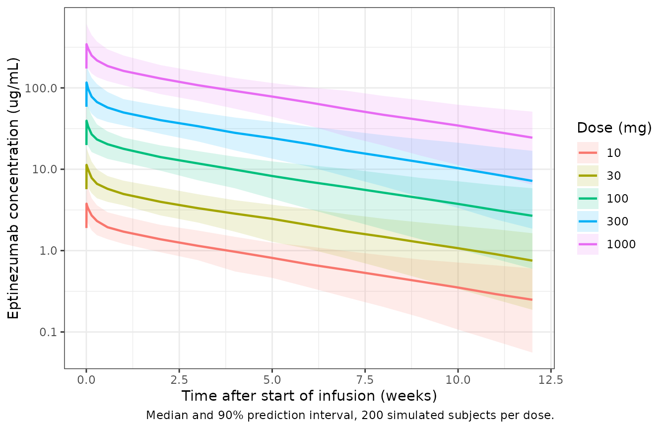

PKNCA: single-dose exposure (Table 2)

AUC0-12wk, Cmax and Cavg are computed over 0-2016 h. Ctrough is the concentration at the end of the 12-week interval, which PKNCA reports as clast.obs because the last sample is at 2016 h. Table 2 reports arithmetic means, so the simulated values are summarised as means before the comparison.

conc <- sim |>
  filter(!is.na(Cc)) |>
  select(id, time, Cc, dose_mg) |>
  mutate(treatment = paste(dose_mg, "mg"))
dose_df <- cohort |>
  transmute(id, time = 0, amt = dose_mg, treatment = paste(dose_mg, "mg"))
conc_obj <- PKNCAconc(conc, Cc ~ time | treatment + id)
dose_obj <- PKNCAdose(dose_df, amt ~ time | treatment + id, route = "intravascular", duration = 1)
intervals <- data.frame(
  start = 0, end = 2016,
  auclast = TRUE, cmax = TRUE, cav = TRUE, clast.obs = TRUE
)
nca <- pk.nca(PKNCAdata(conc_obj, dose_obj, intervals = intervals))

sim_means <- as.data.frame(nca$result) |>
  group_by(treatment, PPTESTCD) |>
  summarise(PPORRES = mean(PPORRES), .groups = "drop")

published <- tribble(
  ~treatment, ~auclast, ~cmax, ~cav, ~clast.obs,
  "10 mg", 2050, 4.32, 1.02, 0.294,
  "30 mg", 5770, 12.4, 2.87, 0.821,
  "100 mg", 17900, 37.3, 8.95, 2.66,
  "300 mg", 54500, 114, 27.2, 8.06,
  "1000 mg", 164000, 348, 81.3, 23.3
)

cmp <- nlmixr2lib::ncaComparisonTable(
  simulated = sim_means,
  reference = published,
  by = "treatment",
  units = c(auclast = "h*ug/mL", cmax = "ug/mL", cav = "ug/mL", clast.obs = "ug/mL"),
  tolerance_pct = 20
)
knitr::kable(cmp, caption = "Simulated vs published (Baker 2020 Table 2) mean single-dose exposure. * differs by >20%.")

Simulated vs published (Baker 2020 Table 2) mean single-dose exposure. * differs by >20%.
NCA parameter	treatment	Reference	Simulated	% diff
Cmax (ug/mL)	10 mg	4.32	4.13	-4.5%
Cmax (ug/mL)	30 mg	12.4	11.8	-4.5%
Cmax (ug/mL)	100 mg	37.3	41.6	+11.4%
Cmax (ug/mL)	300 mg	114	121	+6.3%
Cmax (ug/mL)	1000 mg	348	369	+6.1%
Clast (ug/mL)	10 mg	0.294	0.272	-7.3%
Clast (ug/mL)	30 mg	0.821	0.814	-0.9%
Clast (ug/mL)	100 mg	2.66	2.83	+6.4%
Clast (ug/mL)	300 mg	8.06	8.23	+2.1%
Clast (ug/mL)	1000 mg	23.3	26.2	+12.6%
AUClast (h*ug/mL)	10 mg	2050	1780	-13.2%
AUClast (h*ug/mL)	30 mg	5770	5210	-9.7%
AUClast (h*ug/mL)	100 mg	17900	18200	+1.6%
AUClast (h*ug/mL)	300 mg	54500	52800	-3.1%
AUClast (h*ug/mL)	1000 mg	164000	169000	+3.2%
Cavg (ug/mL)	10 mg	1.02	0.883	-13.4%
Cavg (ug/mL)	30 mg	2.87	2.58	-10.0%
Cavg (ug/mL)	100 mg	8.95	9.02	+0.8%
Cavg (ug/mL)	300 mg	27.2	26.2	-3.7%
Cavg (ug/mL)	1000 mg	81.3	84	+3.3%

attr(cmp, "footnote")
#> NULL

All rows are within 20% of Table 2. The 100 mg Cmax is about 11% high and the 10 and 30 mg AUC and Cavg about 10-13% low. The simulated arms approximate each dose group’s study mix and covariate distributions, which the paper does not tabulate by dose, so differences of this size are expected.

pct <- sim_means |>
  inner_join(
    pivot_longer(published, -treatment, names_to = "PPTESTCD", values_to = "ref"),
    by = c("treatment", "PPTESTCD")
  ) |>
  mutate(pct_diff = 100 * (PPORRES - ref) / ref)
stopifnot(
  # Structural: a mis-read clearance, volume or dose unit shifts every row.
  abs(median(pct$pct_diff)) < 10,
  # Envelope, robust to which arm draws the heaviest or lightest subjects.
  quantile(abs(pct$pct_diff), 0.9) < 25
)

Accumulation (Table 3)

Table 3 reports accumulation ratios of about 1.15 for AUCtau and 1.08 for Cmax with dosing every 12 weeks. For a typical subject these follow from the disposition parameters alone, so the check uses the reference subject and 100 mg every 2016 h for five doses.

typ <- ref |> mutate(id = 1)
ev_md <- bind_rows(
  typ |> tidyr::crossing(time = 2016 * 0:4) |>
    mutate(amt = 100, rate = 100, evid = 1, cmt = "central"),
  typ |> tidyr::crossing(time = sort(unique(c(seq(0, 2016 * 5, by = 24), 2016 * 0:4 + 1)))) |>
    mutate(amt = NA_real_, rate = NA_real_, evid = 0, cmt = "central")
) |> arrange(time, desc(evid))
sim_md <- rxSolve(mod_typ, ev_md, returnType = "data.frame")
#> ℹ omega/sigma items treated as zero: 'etalcl', 'etalvc', 'etalq', 'etalvp'
conc_md <- sim_md |> transmute(id = 1, time, Cc)
dose_md <- ev_md |> filter(evid == 1) |> transmute(id, time, amt)
int_md <- data.frame(
  start = c(0, 2016 * 4), end = c(2016, 2016 * 5),
  auclast = TRUE, cmax = TRUE
)
nca_md <- pk.nca(PKNCAdata(
  PKNCAconc(conc_md, Cc ~ time | id),
  PKNCAdose(dose_md, amt ~ time | id, route = "intravascular", duration = 1),
  intervals = int_md
))
res_md <- as.data.frame(nca_md$result)
rac <- res_md |>
  group_by(PPTESTCD) |>
  summarise(Rac = PPORRES[start == 2016 * 4] / PPORRES[start == 0], .groups = "drop")
knitr::kable(rac, digits = 3, caption = "Typical-subject accumulation ratio; Baker 2020 Table 3 means are 1.13-1.15 (AUC) and 1.08-1.10 (Cmax).")

Typical-subject accumulation ratio; Baker 2020 Table 3 means are 1.13-1.15 (AUC) and 1.08-1.10 (Cmax).
PPTESTCD	Rac
auclast	1.126
cmax	1.080

stopifnot(
  abs(rac$Rac[rac$PPTESTCD == "auclast"] - 1.14) < 0.03,
  abs(rac$Rac[rac$PPTESTCD == "cmax"] - 1.08) < 0.03
)

The typical-subject AUC ratio (1.13) sits at the low end of the Table 3 means (1.13-1.15), which are averages over individuals with between-subject variability; the Cmax ratio (1.08) matches.

Exposure-response models not included

Baker 2020 relates the change in monthly migraine days over weeks 1-12 to exposure with a placebo-anchored inhibitory Emax model, E0 + Imax x AUC/(AUC50 + AUC), fitted separately for EM and CM. Only the EC50 values (Table 4) are published; E0 and Imax are not given in the article, the FDA review (Table 13) or the EMA report (Table 14). The logistic regressions for the 50% and 75% responder rates are published as slopes only (Figure 7), without intercepts. Neither model can be reproduced, so the package contains the population PK model only.

Assumptions and deviations

Source of the covariate coefficients. The journal article names the retained covariates but does not print their coefficients, Q, Vp, the Q/Vp variability or the proportional error. All of these come from the sponsor parameter table reproduced as FDA review Table 12. The article’s own values (CL, Vc, BSV on CL and Vc, additive error, half-lives) agree with that table.
Shared weight exponents. Table 12 prints the weight term on Q and Vp without its own exponent. EMA report Table 6 adds weight on CL and Q as one fitted parameter (step 1) and on Vc and Vp as one fitted parameter (step 2), so Q uses the CL exponent (0.709) and Vp uses the Vc exponent (0.544). The recovered alpha and beta half-lives above confirm the reference values.
EM/CM labels. Table 12 and Figure 4 disagree on which migraine group has the larger CL effect (see the Figure 4 section). The model follows Table 12.
Q-Vp correlation. The base model had a correlated Q-Vp eta block (EMA report Table 6, footnote a), but the covariance is not printed in any source. The etas are independent in this implementation. This affects only the spread of the distribution phase.
Baseline MMD for healthy participants. The paper does not say what value healthy participants carried. They are simulated at the 13-day reference, which matches the typical healthy subject of Figure 4.
Creatinine clearance. The model applies the 150 mL/min cap internally; supply the uncapped Cockcroft-Gault value in mL/min.
Virtual cohort. Weight (log-normal around the median, clipped to the observed range), creatinine clearance (normal, mean 118 mL/min, SD 25), baseline MMD by disease and sex are assumed distributions. The disease mix per dose follows Table 1; all infusions last 1 hour.
Low-dose nonlinearity. The EMA report notes a departure from dose proportionality at 10 mg and below, possibly target-mediated, that the linear model does not describe. Predictions for doses below 10 mg should be read with that in mind.