Tozorakimab (Sadiq 2024)
Source:vignettes/articles/Sadiq_2024_tozorakimab.Rmd
Sadiq_2024_tozorakimab.RmdModel and source
- Citation: Sadiq MW, Yu H, Astrand M, Scott IC, Williams A, Hewitt L, White N, Killick H, Gavala M, Cohen ES, Reid F, Kell C, Pandya H, Jimenez E. Population pharmacokinetic/target engagement modelling of tozorakimab in healthy volunteers and patients with chronic obstructive pulmonary disease. Br J Clin Pharmacol. 2024;90(12):3286-3295. doi:10.1111/bcp.16195.
- Description: Two-compartment population PK / target-engagement model for tozorakimab (anti-IL-33 IgG1 monoclonal antibody) with explicit central-compartment binding of IL-33 to tozorakimab and to the soluble decoy receptor sST2, in healthy adults and patients with mild COPD
- Article: https://doi.org/10.1111/bcp.16195
Tozorakimab is a high-affinity human IgG1 monoclonal antibody that neutralises interleukin-33 (IL-33). Sadiq 2024 couples a two-compartment population PK model for tozorakimab to an explicit ligand-binding target-engagement (TE) layer: free IL-33 is produced at a zero-order rate and is captured either by tozorakimab (forming the IL-33/tozorakimab complex) or by the soluble decoy receptor sST2 (forming the IL-33/sST2 complex, which is the circulating form of IL-33 in serum). Systemic target engagement is read out as the reduction in the IL-33/sST2 complex.
Population
The model was fit to 60 tozorakimab-treated participants from the first-in-human phase 1 study NCT03096795 (Table 1 and Section 2.1). Single ascending dose (SAD) cohorts enrolled healthy adults with mild atopy and house dust mite sensitivity and received 1, 3, 10, 30, 100 or 300 mg subcutaneously (SC) or 300 mg intravenously (IV); multiple ascending dose (MAD) cohorts enrolled adults with GOLD grade I-II chronic obstructive pulmonary disease (COPD) and received 30 or 300 mg SC once every 2 weeks on days 1, 15 and 29; a Japanese cohort of healthy adults received 300 mg IV. Table 1 tabulates 66 tozorakimab-treated participants (42 SAD, 18 MAD, 6 Japanese) with cohort mean body weights of 77.4, 78.4 and 70.4 kg; the analysis set is 60 because the 100 mg MAD cohort was excluded after its PK levels were “consistently lower than expected” with no root cause identified (Section 3.1). Participants were predominantly male (about 14% female across Table 1) and predominantly White (about 73%, with 18% Asian).
Sex, age, race, body weight and study population (healthy volunteer
vs COPD) were screened on clearance and central volume by stepwise
covariate modelling in Perl-speaks-NONMEM; none was
retained (Section 3.3). The model therefore has no covariate
terms, and these screened covariates are recorded in the model file’s
covariatesDataExcluded metadata rather than in
covariateData.
The same information is available programmatically via the model’s
population metadata:
str(readModelDb("Sadiq_2024_tozorakimab")()$population)
#> List of 10
#>  $ species       : chr "human"
#>  $ n_subjects    : num 60
#>  $ n_studies     : num 1
#>  $ disease_state : chr "healthy adults with mild atopy and house dust mite sensitivity (SAD and Japanese cohorts); adults with GOLD gra"| __truncated__
#>  $ weight_median : chr "cohort means 77.4 kg (SAD), 78.4 kg (MAD), 70.4 kg (Japanese)"
#>  $ sex_female_pct: num 13.6
#>  $ race_ethnicity: Named num [1:4] 72.7 18.2 7.6 1.5
#>   ..- attr(*, "names")= chr [1:4] "White" "Asian" "Other" "Black"
#>  $ dose_range    : chr "SAD: 1, 3, 10, 30, 100 or 300 mg SC single dose, or 300 mg IV single dose; MAD: 30 or 300 mg SC once every 2 we"| __truncated__
#>  $ regions       : chr "single first-in-human study (NCT03096795) approved by the London Hampstead Research Ethics Committee; includes "| __truncated__
#>  $ notes         : chr "Baseline demographics are Table 1, which tabulates 66 tozorakimab-treated participants (42 SAD, 18 MAD, 6 Japan"| __truncated__
Source trace
Every ini() entry in
inst/modeldb/specificDrugs/Sadiq_2024_tozorakimab.R carries
an in-file comment naming its source location. They are collected here
for review.
| Equation / parameter | Value | Source location |
|---|---|---|
lka (Ka) |
0.48 1/day | Table 2 (RSE 10.11%) |
lcl (CL) |
0.87 L/day | Table 2 (RSE 14.89%) |
lvc (Vc) |
12.64 L | Table 2 (RSE 19.91%) |
lvp (Vp) |
2.61 L, fixed | Table 2 |
lq (Q) |
0.21 L/day, fixed | Table 2 |
lfdepot (Fsc) |
0.45 | Table 2 (RSE 10.08%) |
lkdeg (Kel,IL-33) |
4.83 1/day | Table 2 (RSE 45.94%) |
lkdeg_sst2 (Kel,sST2) |
0.069 1/day | Table 2 (RSE 22.54%) |
lkon (Kon,IL-33/tozo) |
68.85 1/nM/day | Table 2 (RSE 29.07%) |
lkon_sst2 (Kon,IL-33/sST2) |
91.38 1/nM/day | Table 2 (RSE 23.57%) |
lkd (Kd,IL-33/tozo) |
3e-05 nM, fixed | Table 2 |
lkd_sst2 (Kd,IL-33/sST2) |
6e-04 nM, fixed | Table 2 |
lbl_sst2 (BL,sST2) |
0.20 nM, fixed | Table 2 |
lbl_complex_sst2 (BL,IL-33/sST2) |
0.00047 nM | Table 2 (RSE 5.29%) |
| IIV on CL, Kon,IL-33/tozo, Kel,sST2, Kon,IL-33/sST2, BL,IL-33/sST2, Fsc | 20.79 / 72.51 / 51.47 / 45.72 / 30.02 / 32.23 CV% | Table 2; converted with the table note
variance = log(CV^2 + 1)
|
propSd, propSd_complex,
propSd_Cc_complex_sst2
|
9.97 / 5.14 / 1.06 (%) | Table 2 residual-error rows; see Assumptions |
d/dt(central), d/dt(peripheral1)
|
n/a | Section 2.2, “Free tozorakimab concentration in the central / peripheral compartment” |
d/dt(target) (free IL-33) and Kin,IL-33 |
n/a | Section 2.2, “Free IL-33 concentration” |
d/dt(sst2) (free sST2) and Kin,sST2 |
n/a | Section 2.2, “Free sST2 concentration”; see Assumptions |
d/dt(complex) (IL-33/tozorakimab) |
n/a | Section 2.2, “IL-33/tozorakimab complex concentration” |
d/dt(complex_sst2) (IL-33/sST2) |
n/a | Section 2.2, “IL-33/sST2 complex concentration” |
| Model diagram (elimination routes, binding topology) | n/a | Figure 1 |
Units and the molar-mass assumption
The model is molar throughout: every TE parameter in Table 2 carries molar units (Kon in 1/nM/day, Kd and both baselines in nM), so the free-tozorakimab state that multiplies Kon must also be in nM. Doses are therefore given in nmol and all states are in nM.
The paper reports doses in mg and concentrations in ug/mL (tozorakimab, Figure 2) or pg/mL (both complexes, Figures 3 and 4), but never reports the molar masses needed to convert. Reproducing the published figures on their own axes therefore requires one non-paper value: the molar mass of tozorakimab. A typical human IgG1 (146 kDa) is assumed below, and the assumption is tested rather than merely asserted – see the Assumptions section.
Endpoints that do not need a molar mass are preferred wherever possible: systemic target engagement is reported as percent inhibition of the IL-33/sST2 complex relative to its own baseline, which is exactly the quantity the paper simulates in Figure 5 and is unit-free.
MW_TOZ <- 146000                       # g/mol; assumed human IgG1 (NOT from the paper)
nmol_from_mg  <- function(mg) mg / MW_TOZ * 1e6
ugml_from_nM  <- function(nM) nM * MW_TOZ / 1e6
Virtual cohort
Original observed data are not publicly available. The cohorts below reproduce the published dosing regimens; the model carries no covariates, so no covariate distribution has to be simulated.
set.seed(20241129)
N_ARM <- 100                            # per arm; well under the 200/arm cap

# The grid must contain the dosing-interval boundaries (days 14, 28, 42) so the
# accumulation-ratio AUCs below are computed over complete, matched intervals.
obs_times <- sort(unique(c(seq(0, 15, by = 1), seq(16, 48, by = 2),
                          seq(50, 169, by = 3))))
stopifnot(all(c(0, 14, 28, 42) %in% obs_times))

# Observation rows carry cmt = NA + dvid = 1 because all three endpoints
# (Cc, Cc_complex, Cc_complex_sst2) are algebraic observables, not ODE states.
make_arm <- function(arm, dose_mg, cmt, ii = 0, addl = 0L, id_offset = 0L,
                     times = obs_times) {
  ids <- id_offset + seq_len(N_ARM)
  dz <- tibble(id = ids, time = 0, evid = 1L, amt = nmol_from_mg(dose_mg),
               cmt = cmt, dvid = NA_integer_, ii = ii, addl = addl)
  ob <- tibble(id = rep(ids, each = length(times)),
               time = rep(times, times = N_ARM), evid = 0L, amt = NA_real_,
               cmt = NA_character_, dvid = 1L, ii = 0, addl = 0L)
  bind_rows(dz, ob) |>
    mutate(arm = arm) |>
    arrange(id, time, desc(evid))
}

events <- bind_rows(
  make_arm("30 mg SC (SAD)",       30,  "depot",   id_offset =   0L),
  make_arm("300 mg SC (SAD)",     300,  "depot",   id_offset = 100L),
  make_arm("300 mg IV (SAD)",     300,  "central", id_offset = 200L),
  make_arm("300 mg SC Q2W (MAD)", 300,  "depot",   ii = 14, addl = 2L,
           id_offset = 300L)
)
stopifnot(!anyDuplicated(events[events$evid == 0L, c("id", "time")]))
Simulation
mod <- readModelDb("Sadiq_2024_tozorakimab")

sim <- rxode2::rxSolve(mod, events = events, keep = "arm") |>
  as.data.frame() |>
  mutate(
    arm      = factor(arm, levels = c("30 mg SC (SAD)", "300 mg SC (SAD)",
                                      "300 mg IV (SAD)", "300 mg SC Q2W (MAD)")),
    Cc_ugml  = ugml_from_nM(Cc),
    # percent inhibition of the IL-33/sST2 complex relative to the subject's
    # own simulated baseline -- unit-free, no molar mass required
    te_pct   = 100 * (1 - Cc_complex_sst2 / bl_complex_sst2)
  )
#> ℹ parameter labels from comments will be replaced by 'label()'
Structural check: the untreated system holds at baseline
The TE layer is a steady-state-balance model: with no drug present,
free IL-33, free sST2 and the IL-33/sST2 complex must sit exactly at
their baselines indefinitely. This is the sharpest available test of the
two zero-order input relations (Kin,IL-33 and
Kin,sST2) and of the baseline free-IL-33 derivation, all of
which are reconstructions of printed relations.
mod_typ <- rxode2::zeroRe(readModelDb("Sadiq_2024_tozorakimab"))
#> ℹ parameter labels from comments will be replaced by 'label()'
no_dose <- tibble(id = 1L, time = seq(0, 400, by = 5), evid = 0L,
                  amt = NA_real_, cmt = NA_character_, dvid = 1L,
                  ii = 0, addl = 0L)
hold <- rxode2::rxSolve(mod_typ, events = no_dose) |> as.data.frame()
#> ℹ omega/sigma items treated as zero: 'etalcl', 'etalkon', 'etalkdeg_sst2', 'etalkon_sst2', 'etalbl_complex_sst2', 'etalfdepot'

baseline_drift <- tibble(
  species = c("free IL-33 (target)", "free sST2", "IL-33/sST2 complex"),
  baseline_nM = c(hold$bl_target[1], hold$bl_sst2[1], hold$bl_complex_sst2[1]),
  `max relative drift over 400 days` = c(
    max(abs(hold$target       - hold$bl_target[1]))       / hold$bl_target[1],
    max(abs(hold$sst2         - hold$bl_sst2[1]))         / hold$bl_sst2[1],
    max(abs(hold$complex_sst2 - hold$bl_complex_sst2[1])) / hold$bl_complex_sst2[1]
  )
)
knitr::kable(baseline_drift, digits = c(0, 8, 12),
caption = "Baseline hold with no dose. Drift at integrator tolerance confirms the reconstructed zero-order input relations.")| species | baseline_nM | max relative drift over 400 days |
|---|---|---|
| free IL-33 (target) | 3.18e-06 | 0 |
| free sST2 | 2.00e-01 | 0 |
| IL-33/sST2 complex | 4.70e-04 | 0 |
Replicate published figures
# Replicates Figure 2 of Sadiq 2024: pcVPC of serum tozorakimab concentration
# by cohort. Axis converted to ug/mL with the assumed IgG1 molar mass.
sim |>
  filter(Cc_ugml > 0) |>
  group_by(arm, time) |>
  summarise(Q05 = quantile(Cc_ugml, 0.05), Q50 = median(Cc_ugml),
            Q95 = quantile(Cc_ugml, 0.95), .groups = "drop") |>
  ggplot(aes(time, Q50)) +
  geom_ribbon(aes(ymin = Q05, ymax = Q95), alpha = 0.25) +
  geom_line() +
  geom_hline(yintercept = 0.01, linetype = "dashed") +
  facet_wrap(~arm) +
  scale_y_log10() +
  labs(x = "Time after first dose (days)",
       y = "Tozorakimab concentration (ug/mL)",
       title = "Figure 2 - simulated tozorakimab PK by cohort",
       caption = "Replicates Figure 2 of Sadiq 2024. Dashed line is the 0.01 ug/mL LLOQ.")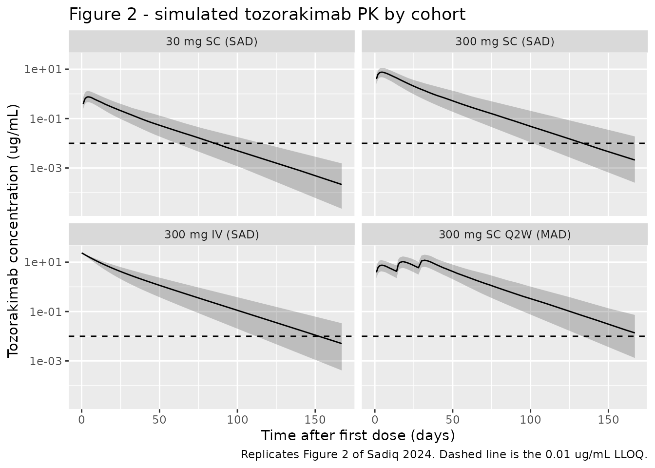
# Replicates Figure 3 of Sadiq 2024: IL-33/sST2 complex over time, shown as
# percent of each subject's own baseline (the paper plots pg/mL).
sim |>
  filter(!is.na(Cc)) |>
  group_by(arm, time) |>
  summarise(Q05 = quantile(te_pct, 0.05), Q50 = median(te_pct),
            Q95 = quantile(te_pct, 0.95), .groups = "drop") |>
  ggplot(aes(time, Q50)) +
  geom_ribbon(aes(ymin = Q05, ymax = Q95), alpha = 0.25) +
  geom_line() +
  facet_wrap(~arm) +
  labs(x = "Time after first dose (days)",
       y = "Inhibition of the IL-33/sST2 complex (% of baseline)",
       title = "Figure 3 - simulated systemic target engagement",
       caption = "Replicates the shape of Figure 3 of Sadiq 2024 (there plotted as pg/mL); inhibition is 100% minus the plotted fraction of baseline.")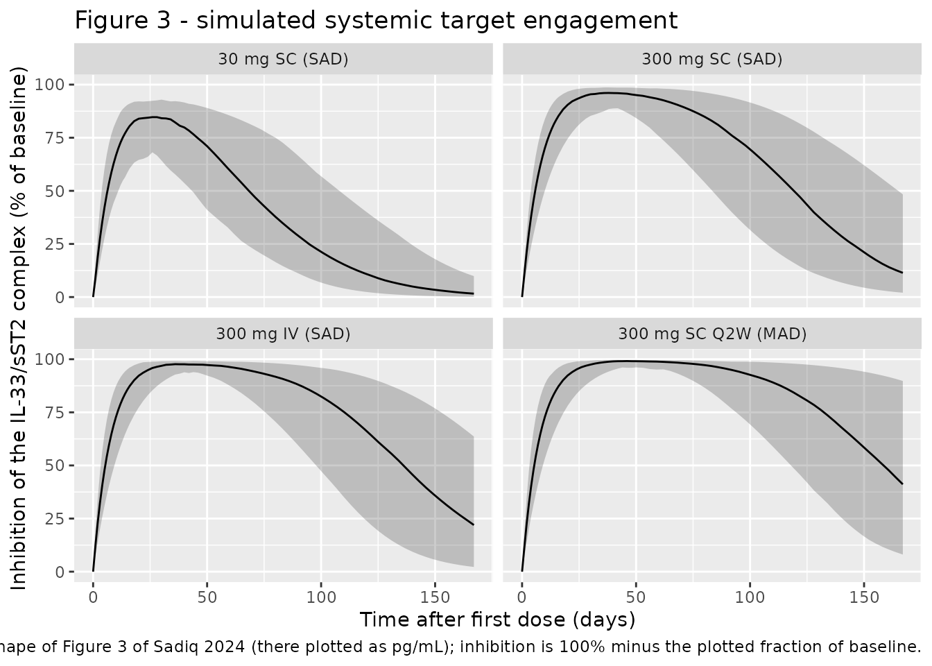
# Replicates Figure 4 of Sadiq 2024: IL-33/tozorakimab complex over time.
# Left in nM: the paper plots pg/mL but reports no molar mass for the complex.
sim |>
  filter(!is.na(Cc)) |>
  group_by(arm, time) |>
  summarise(Q05 = quantile(Cc_complex, 0.05), Q50 = median(Cc_complex),
            Q95 = quantile(Cc_complex, 0.95), .groups = "drop") |>
  ggplot(aes(time, Q50)) +
  geom_ribbon(aes(ymin = Q05, ymax = Q95), alpha = 0.25) +
  geom_line() +
  facet_wrap(~arm) +
  labs(x = "Time after first dose (days)",
       y = "IL-33/tozorakimab complex (nM)",
       title = "Figure 4 - simulated IL-33/tozorakimab complex",
       caption = "Replicates Figure 4 of Sadiq 2024 (there plotted as pg/mL).")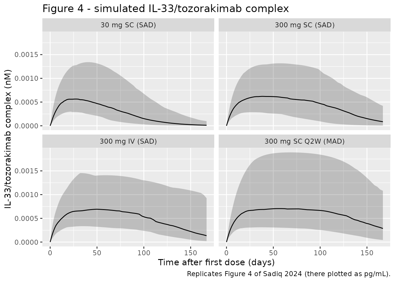
The simulated IL-33/tozorakimab complex rises to a plateau and decays slowly, and the IL-33/sST2 complex falls with a delay relative to the tozorakimab peak and recovers late – both consistent with the Discussion’s explanation that “the maximum inhibition of IL-33/sST2 is dependent on the clearance of already formed IL-33/sST2 complexes, because tozorakimab is not anticipated to displace sST2 from already formed IL-33/sST2 complexes”.
Figure 5: target engagement at steady-state trough
# Replicates Figure 5 of Sadiq 2024: inhibition of the IL-33/sST2 complex at
# trough PK at steady state, across seven doses and three dose frequencies.
N_TE  <- 50
doses <- c(30, 60, 90, 120, 150, 300, 600)
regs  <- c(Q2W = 14, Q4W = 28, Q6W = 42)

te_arm <- function(dose_mg, tau, id_offset) {
  k   <- ceiling(420 / tau)
  ids <- id_offset + seq_len(N_TE)
  bind_rows(
    tibble(id = ids, time = 0, evid = 1L, amt = nmol_from_mg(dose_mg),
           cmt = "depot", dvid = NA_integer_, ii = tau, addl = k),
    tibble(id = ids, time = k * tau, evid = 0L, amt = NA_real_,
           cmt = NA_character_, dvid = 1L, ii = 0, addl = 0L)
  ) |>
    mutate(dose_mg = dose_mg, regimen = names(regs)[match(tau, regs)]) |>
    arrange(id, time, desc(evid))
}

grid_te  <- expand_grid(dose_mg = doses, tau = unname(regs))
ev_te <- bind_rows(Map(te_arm, grid_te$dose_mg, grid_te$tau,
                       (seq_len(nrow(grid_te)) - 1L) * N_TE))

sim_te <- rxode2::rxSolve(mod, events = ev_te,
                          keep = c("dose_mg", "regimen")) |>
  as.data.frame() |>
  filter(!is.na(Cc)) |>
  mutate(te_pct = 100 * (1 - Cc_complex_sst2 / bl_complex_sst2))

te_summary <- sim_te |>
  group_by(regimen, dose_mg) |>
  summarise(median_inhibition = median(te_pct), .groups = "drop") |>
  mutate(regimen = factor(regimen, levels = c("Q2W", "Q4W", "Q6W")))

ggplot(te_summary, aes(dose_mg, median_inhibition, colour = regimen)) +
  geom_line() + geom_point() +
  geom_hline(yintercept = 95, linetype = "dashed") +
  scale_x_continuous(breaks = doses) +
  coord_cartesian(ylim = c(75, 100)) +
  labs(x = "Tozorakimab dose (mg SC)",
       y = "Median inhibition of IL-33/sST2 at steady-state trough (%)",
       colour = "Regimen",
       title = "Figure 5 - target engagement at steady-state trough",
       caption = "Replicates Figure 5 of Sadiq 2024. Dashed line is the paper's 95% threshold.")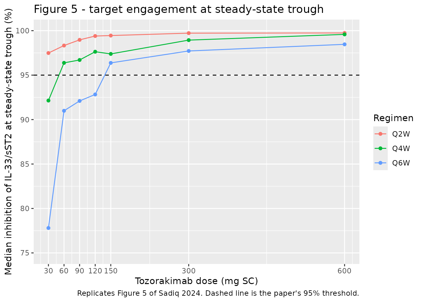
te_summary |>
  pivot_wider(names_from = regimen, values_from = median_inhibition) |>
  arrange(dose_mg) |>
  rename("Dose (mg SC)" = dose_mg) |>
  knitr::kable(digits = 1,
caption = "Median percent inhibition of the IL-33/sST2 complex at steady-state trough.")| Dose (mg SC) | Q2W | Q4W | Q6W |
|---|---|---|---|
| 30 | 97.5 | 92.1 | 77.8 |
| 60 | 98.3 | 96.4 | 91.0 |
| 90 | 99.0 | 96.7 | 92.1 |
| 120 | 99.4 | 97.6 | 92.8 |
| 150 | 99.5 | 97.4 | 96.4 |
| 300 | 99.7 | 98.9 | 97.7 |
| 600 | 99.7 | 99.6 | 98.5 |
The paper reports that “for all three regimens, IL-33/sST2 complex inhibition was more than 95% at doses greater than 90 mg”. The simulation reproduces this for Q2W and Q4W. For Q6W the median crosses 95% only at about 150 mg; see Assumptions.
PKNCA validation
NCA is run on the three single-dose SAD arms. Concentrations are converted to ug/mL so that the derived exposures are on the paper’s reporting scale.
sd_arms <- c("30 mg SC (SAD)", "300 mg SC (SAD)", "300 mg IV (SAD)")

sim_nca <- sim |>
  filter(arm %in% sd_arms) |>
  transmute(id, time, arm = as.character(arm), Cc = Cc_ugml) |>
  filter(!is.na(Cc))

# Guarantee a time = 0 record per (id, arm).
sim_nca <- bind_rows(
  sim_nca,
  sim_nca |> distinct(id, arm) |> mutate(time = 0, Cc = 0)
) |>
  distinct(id, arm, time, .keep_all = TRUE) |>
  arrange(id, arm, time)

conc_obj <- PKNCA::PKNCAconc(sim_nca, Cc ~ time | arm + id)

dose_df <- events |>
  filter(evid == 1, arm %in% sd_arms) |>
  transmute(id, time, amt, arm = as.character(arm))

dose_obj <- PKNCA::PKNCAdose(dose_df, amt ~ time | arm + id)

intervals <- data.frame(start = 0, end = Inf,
                        cmax = TRUE, tmax = TRUE,
                        aucinf.obs = TRUE, half.life = TRUE)

nca_res <- PKNCA::pk.nca(PKNCA::PKNCAdata(conc_obj, dose_obj,
                                          intervals = intervals))
Comparison against published NCA
Sadiq 2024 does not tabulate per-dose NCA. It reports a mean terminal half-life of 11.7-17.3 days across all cohorts (Section 3.2, citing the phase 1 report). The comparison below anchors every arm on the midpoint of that range, 14.5 days; the midpoint is a comparison anchor chosen here, not a value the paper states. Cmax and AUC have no published counterparts, so they are shown as simulated values only.
published <- tibble::tribble(
  ~arm,               ~half.life,
  "30 mg SC (SAD)",   14.5,
  "300 mg SC (SAD)",  14.5,
  "300 mg IV (SAD)",  14.5
)

cmp <- nlmixr2lib::ncaComparisonTable(
  simulated     = nca_res,
  reference     = published,
  by            = "arm",
  units         = c(cmax = "ug/mL", aucinf.obs = "day*ug/mL",
                    tmax = "day", half.life = "day"),
  tolerance_pct = 20
)

knitr::kable(cmp, digits = 3,
caption = "Simulated vs published NCA. * differs from the reference by >20%. Published half-life is the 11.7-17.3 day range midpoint reported in Section 3.2; Cmax/Tmax/AUC have no published counterpart.")| NCA parameter | arm | Reference | Simulated | % diff |
|---|---|---|---|---|
| t½ (day) | 30 mg SC (SAD) | 14.5 | 14.3 | -1.1% |
| t½ (day) | 300 mg SC (SAD) | 14.5 | 14.7 | +1.2% |
| t½ (day) | 300 mg IV (SAD) | 14.5 | 14.9 | +2.7% |
Dose proportionality and bioavailability
The paper states that tozorakimab showed “linear and time-independent serum PK” (Section 3.2) and that SC bioavailability was 45% (Table 2, and “consistent with the observed value”, Section 3.3). Both are checkable from the NCA output.
auc_by_arm <- as.data.frame(nca_res) |>
  filter(PPTESTCD == "aucinf.obs") |>
  group_by(arm) |>
  summarise(auc = median(PPORRES), .groups = "drop")

auc_of <- function(a) auc_by_arm$auc[auc_by_arm$arm == a]

checks <- tibble(
  Check = c("Dose proportionality, 300 mg SC / 30 mg SC (expect 10)",
            "Absolute bioavailability, AUC 300 mg SC / AUC 300 mg IV (Table 2: 0.45)"),
  Simulated = c(auc_of("300 mg SC (SAD)") / auc_of("30 mg SC (SAD)"),
                auc_of("300 mg SC (SAD)") / auc_of("300 mg IV (SAD)")),
  Reference = c(10, 0.45)
) |>
  mutate(`Difference (%)` = 100 * (Simulated - Reference) / Reference)

knitr::kable(checks, digits = 3,
caption = "Dose-proportionality and bioavailability gates.")| Check | Simulated | Reference | Difference (%) |
|---|---|---|---|
| Dose proportionality, 300 mg SC / 30 mg SC (expect 10) | 10.222 | 10.00 | 2.216 |
| Absolute bioavailability, AUC 300 mg SC / AUC 300 mg IV (Table 2: 0.45) | 0.451 | 0.45 | 0.265 |
Accumulation ratio
The phase 1 report observed an accumulation ratio (steady-state AUC over a dosing interval divided by first-interval AUC) of 1.6, range 1.2-3.7, in the COPD Q2W cohorts (Section 3.2).
mad <- sim |> filter(arm == "300 mg SC Q2W (MAD)")
sad <- sim |> filter(arm == "300 mg SC (SAD)")

trapz <- function(t, y) sum(diff(t) * (head(y, -1) + tail(y, -1)) / 2)

auc_tau <- function(df, t0, t1) {
  df |>
    filter(time >= t0, time <= t1) |>
    group_by(id) |>
    summarise(auc = trapz(time, Cc), .groups = "drop")
}

acc <- median(auc_tau(mad, 28, 42)$auc) / median(auc_tau(sad, 0, 14)$auc)

knitr::kable(
  tibble(Check = "Accumulation ratio, 300 mg SC Q2W (third interval / first interval)",
         Simulated = acc, `Reference (Section 3.2)` = 1.6,
         `Reference range` = "1.2-3.7"),
  digits = 2,
caption = "Accumulation ratio gate.")| Check | Simulated | Reference (Section 3.2) | Reference range |
|---|---|---|---|
| Accumulation ratio, 300 mg SC Q2W (third interval / first interval) | 1.65 | 1.6 | 1.2-3.7 |
Assumptions and deviations
Two printed relations were reconstructed. The published PDF prints the target-engagement system in Section 2.2. Two of those printed expressions are internally inconsistent with the rest of the system, and both were corrected to the unique form that holds the untreated system exactly at baseline (verified in the “Structural check” section above, where drift is at integrator tolerance):
-
Free sST2 equation. As printed, the dissociation term
enters with a minus sign (
- Koff,IL-33/sST2 * IL-33/sST2). Dissociation of the IL-33/sST2 complex releases free sST2, so the term must be positive. With the printed sign the untreated system cannot be at steady state. -
Kin,sST2. As printed this reads
Kin,sST2 = Kel,IL-33 * (BL_IL-33 + BL_IL-33/sST2)– i.e. an sST2 input rate built from IL-33 quantities. Substituting the tabulated values gives 0.00229 nM/day against the 0.01383 nM/day the sST2 balance requires, a 6-fold mismatch. The subscript-consistent formKin,sST2 = Kel,sST2 * (BL_sST2 + BL_IL-33/sST2)reproduces the required value exactly. The printed form appears to be a subscript error.
The IL-33 equation, its Kin,IL-33 relation, both complex
equations and both tozorakimab equations were used exactly as
printed.
Kd is an equilibrium constant, not an
off-rate. Table 2’s abbreviation list glosses Kd
as “dissociation rate constant”, but the model requires the off-rates
Koff = Kd * Kon. Read as rate constants the tabulated
values (3e-05 and 6e-04 per day) would imply off-rate half-lives of
decades; read as equilibrium constants they are 30 pM and 600 pM, which
are textbook affinities and reproduce the Discussion’s statement that
IL-33 binds tozorakimab preferentially over sST2 (a 20-fold affinity
difference). Only the equilibrium reading reproduces the paper’s own
dose-response claim in Figure 5.
Baseline free IL-33 is derived, not tabulated. Table
2 does not report BL_IL-33, which the printed Kin,IL-33
relation needs. It is obtained by setting the printed IL-33/sST2 complex
equation to zero at baseline:
BL_IL-33 = (Koff,IL-33/sST2 + Kel,sST2) * BL_IL-33/sST2 / (Kon,IL-33/sST2 * BL_sST2),
giving 3.18e-06 nM.
Peripheral tozorakimab state. The printed peripheral
equation is
d(tozo_peri)/dt = (Q/Vcent)*tozo_free - (Q/Vperi)*tozo_peri,
which is not mass conserving if tozo_peri is read as the
peripheral concentration. It is exactly mass conserving if
tozo_peri denotes the peripheral amount divided by the
central volume, which is the standard NONMEM scaling. The model
file encodes the equivalent amount-based form, which reproduces the
printed equations term for term.
Residual error: proportional only. Table 2’s six
residual rows are all labelled “(%)” with no units and are NONMEM
$SIGMA variances, not standard deviations. Read as standard
deviations the additive terms are physically impossible: 482.11 against
an IL-33/tozorakimab complex that never exceeds about 40 pg/mL in Figure
4, and 31.51 against an IL-33/sST2 baseline of about 26 pg/mL in Figure
3. Read as variances they give additive SDs of 22.0 and 5.6 pg/mL, which
match the scatter in those figures. The proportional terms are
scale-free and are encoded as
propSd = sqrt(reported% / 100), giving residual CVs of
31.6%, 22.7% and 10.3% – large values that are consistent with 23.7% of
PK samples having been imputed at half the LLOQ (Section 3.3). The
additive terms carry the paper’s ug/mL and pg/mL
reporting units and cannot be converted to this model’s nM states
without molar masses the paper never reports, so they are
not encoded. Anyone needing them should add them on the
reporting scale with an explicit molar mass.
Molar mass of tozorakimab (146 kDa) is not from the paper. It is needed only to place doses and concentrations on the paper’s mg and ug/mL axes; the model itself is molar and needs no molar mass. Two independent checks support a value in the IgG1 range: the simulated terminal half-life and bioavailability gates above are molar-mass free and pass, while the Figure 5 target-engagement threshold (95% inhibition at 90 mg Q4W) and the Figure 2 peak concentration for 300 mg SC are only reproduced with a molar mass near 146 kDa. Users dosing in nmol are unaffected by this assumption.
Q6W target engagement is the one quantitative divergence. The paper states that inhibition exceeds 95% at doses above 90 mg for all three regimens; the simulation reproduces this for Q2W and Q4W but reaches 95% only near 150 mg for Q6W (92.4% at 90 mg, 94.4% at 120 mg). No parameter was adjusted to close the gap. The most likely contributors are the 146 kDa molar-mass assumption, which scales the molar trough concentration directly, and the fact that the paper’s Figure 5 summarises 5000 virtual individuals whereas this vignette uses 50 per arm.
The IL-33/sST2 complex elimination rate is
Kel,sST2. Figure 1 labels that arrow
Kel,IL-33/sST2, suggesting a distinct constant, but Table 2
contains no such parameter and the printed complex equation uses
Kel,sST2. The equation was followed, and the baseline-hold
check confirms it.
Supplement not available. The supporting information (Figures S1-S3) holds goodness-of-fit plots only and contains no parameter values; nothing needed by the model is missing from the main article.
No covariates. The model has no covariate terms
because none survived the paper’s stepwise covariate screen (Section
3.3). The screened covariates are documented in the model file’s
covariatesDataExcluded metadata.
Lognormal IIV on bioavailability. Fsc
carries lognormal IIV of 32.23 CV% as reported, so a small fraction of
simulated individuals (about 0.5%) has F > 1. This is
faithful to the published parameterisation, not a modelling choice made
here.