Pregabalin-Sildenafil Interaction in Rats (Bender 2009)
Source:vignettes/articles/Bender_2009_pregabalin_rat.Rmd
Bender_2009_pregabalin_rat.RmdModel and source
- Citation (binary form): Bender G, Gosset J, Florian J, Tan K, Field M, Marshall S, DeJongh J, Bies R, Danhof M. (2009). Population pharmacokinetic model of the pregabalin-sildenafil interaction in rats: Application of simulation to preclinical PK-PD study design. Pharmaceutical Research 26(10):2259-2269. doi:10.1007/s11095-009-9942-y.
- Description (binary form): Preclinical (rat). Two-compartment population PK model for pregabalin in male Sprague-Dawley rats following a 2 h intravenous infusion (4 or 10 mg/kg/h) in a chronic- constriction-injury (CCI) neuropathic-pain model, with the concomitant administration of sildenafil encoded as a BINARY presence indicator (CONMED_SILDENAFIL). Sildenafil presence reduces pregabalin clearance by a fixed fraction (theta_SLD = 0.302, i.e. 30.2% reduction) per the paper’s discrete-covariate parameterisation; the alternative continuous saturable-metabolite parameterisation is encoded in the companion file Bender_2009_pregabalin_rat_smetab.R. Crossover design with two occasions per rat (Day 1 / Day 4 with a washout) carries between-occasion variability on CL and Vc multiplexed by the OCC indicator. Parameter values from Bender 2009 Table IV (Binary Sildenafil Covariate column).
- Description (continuous-metabolite form): Preclinical (rat). Two-compartment population PK model for pregabalin in male Sprague-Dawley rats following a 2 h intravenous infusion (4 or 10 mg/kg/h) in a chronic- constriction-injury (CCI) neuropathic-pain model, with the concomitant administration of sildenafil encoded as a CONTINUOUS saturable inhibition driven by the time-varying plasma concentration of sildenafil’s active N-methyl metabolite (SLDM). Effective CL = theta_CL * (1 - SLDM / (theta_SLD + SLDM)) with theta_SLD = 1350 ng/mL acting as the IC50 of metabolite-driven inhibition. Statistically the preferred parameterisation in the paper (delta-OFV = -42.6 vs the no-covariate base; the simpler binary form is in the companion file Bender_2009_pregabalin_rat_binary.R with delta-OFV = -8.5). Crossover design with two occasions per rat (Day 1 / Day 4 with a washout) carries between-occasion variability on CL and Vc multiplexed by the OCC indicator. Parameter values from Bender 2009 Table IV (Continuous Sildenafil Metabolite Covariate column).
- Article: https://doi.org/10.1007/s11095-009-9942-y
Bender 2009 develops a two-compartment population PK model for pregabalin in male Sprague-Dawley rats and quantifies the pharmacokinetic drug-drug interaction (DDI) effect of co-administered sildenafil on pregabalin clearance. The structural disposition is a NONMEM ADVAN3 / TRANS4 two-compartment IV model fit with FOCE-I to a two-day crossover dataset. Two competing covariate parameterisations for the sildenafil effect on pregabalin clearance are reported in Table IV and presented as alternative final models:
-
Binary form
(
Bender_2009_pregabalin_rat_binary): a single per-occasion indicator SLDB in {0, 1} reduces typical clearance by the fixed fraction theta_SLD = 0.302 (30.2% reduction when sildenafil is co-administered). This is the parameterisation highlighted in the paper’s abstract. -
Continuous-metabolite form
(
Bender_2009_pregabalin_rat_smetab): the time-varying plasma concentration of sildenafil’s active N-methyl metabolite [SLDM] drives a saturable inhibition function on clearance,CL = theta_CL * (1 - SLDM / (theta_SLD + SLDM)), with the IC50 theta_SLD = 1350 ng/mL. This form has the larger objective-function drop in the LRT (Delta-OFV = 42.6 vs the no-covariate base versus 8.5 for the binary form; the paper’s stated chi-square threshold for df = 1 at p < 0.001 is 10.8, so the metabolite form is the only one that clears the threshold).
This vignette validates both packaged models against the paper’s Figure 2 (raw pregabalin profiles) and Figure 4 (sildenafil effect on clearance), and provides PKNCA NCA estimates for the four study arms.
Choosing between the two parameterisations
The two model files are independent and have the same disposition parameters within numerical precision (Table IV columns are side-by-side); only the covariate term differs. Choose the binary form when the downstream simulation supplies a per-occasion sildenafil presence indicator and you do not have a metabolite concentration profile; choose the continuous-metabolite form when you have or can construct a time-varying [SLDM] profile and want the inhibition to scale with the metabolite concentration. The continuous form is the statistically preferred description per the paper’s LRT but it requires more covariate-column infrastructure to use.
| Property | Binary | Continuous-metabolite |
|---|---|---|
| Covariate column |
CONMED_SILDENAFIL in {0, 1} per occasion |
SLDM (ng/mL), time-varying |
| Effect form | CL *= (1 - 0.302 * CONMED_SILDENAFIL) |
CL *= (1 - SLDM / (1350 + SLDM)) |
| Inhibition at typical sildenafil exposure | flat 30.2% | ~60% at Cmax_SLDM ~ 2100 ng/mL, less between bolus and steady state |
| Delta-OFV vs base | -8.5 (below 10.8 threshold) | -42.6 (above threshold) |
| Recommended use | downstream simulators with only a DDI indicator column | trial simulation with a sildenafil PK model attached |
Population
Bender 2009 used 28 male Sprague-Dawley rats (200-250 g at receipt; Charles River Laboratories, Margate, UK) prepared with the chronic constriction injury (CCI) model of neuropathic pain (Bennett & Xie): four loose ligatures around the right sciatic nerve produced a peripheral mononeuropathy with static and dynamic allodynia. Each rat received a 2 h pregabalin IV infusion through a jugular venous catheter on two experimental days (Day 1 and Day 4, >= 3-day washout) in a crossover design (Table I): four groups of seven rats each received the 4 and 10 mg/kg/h dose levels in randomised order, with co-administered saline or sildenafil 2 mg/kg bolus + 12 mg/kg/h x 6 h infusion. Blood samples were drawn through a carotid artery catheter at sparse D-optimal-selected times between 0.33 and 22 h (Table II). Plasma was analysed by LC-MS/MS for pregabalin (LLOQ 70 ng/mL), sildenafil, and the N-methyl sildenafil metabolite (LLOQ 1 ng/mL each; linear over 5-2,000 ng/mL).
Body weight, age, time post CCI-surgery, and time post catheterization surgery were tested as continuous PK covariates but were not retained – the cohort was intentionally homogeneous (inbred strain, controlled housing), so only sildenafil exposure had a significant impact on OFV.
The same metadata is available programmatically:
readModelDb("Bender_2009_pregabalin_rat_binary")$population.
Source trace
Per-parameter origin (recorded as in-file comments next to each
ini() entry in
inst/modeldb/specificDrugs/Bender_2009_pregabalin_rat_binary.R
and _smetab.R).
Binary form (Bender_2009_pregabalin_rat_binary)
| Equation / parameter | Value | Source location |
|---|---|---|
lcl (log CL) |
log(0.052) | Table IV Binary Sildenafil column: CL = 0.052 L/h, RSE 14.59% |
lvc (log V1) |
log(0.271) | Table IV: V1 = 0.271 L, RSE 3.38% |
lq (log Q) |
log(0.0151) | Table IV: Q = 0.0151 L/h, RSE 35.76% |
lvp (log V2) |
log(2.77) | Table IV: V2 = 2.77 L, RSE 51.99% |
e_sild_cl (theta_SLD, proportional CL reduction) |
0.302 | Table IV: theta_SLD = 0.302, RSE 23.05%; 30.2% CL reduction when SLDB = 1 |
etalcl (BSV CL) |
0.017 (variance) | Table IV: omega^2_1 CL = 0.017, RSE 15.91% |
etalvc (BSV V1) |
0.018 (variance) | Table IV: omega^2_1 V1 = 0.018, RSE 9.26% |
etalq (BSV Q) |
0.439 (variance) | Table IV: omega^2_1 Q = 0.439, RSE 40.87% (Q poorly identified in this model) |
etaiov_cl_1..2 (BOV CL) |
0.061 (variance) | Table IV: omega^2_2 CL = 0.061, RSE 19.52%; occasion 2 fixed equal
per $OMEGA BLOCK(1) SAME
|
etaiov_vc_1..2 (BOV V1) |
0.015 (variance) | Table IV: omega^2_2 V1 = 0.015, RSE 8.75%; occasion 2 fixed equal
per $OMEGA BLOCK(1) SAME
|
propSd |
0.1703 | Table IV: sigma^2 = 0.029, RSE 18.53%; SD = sqrt(0.029) |
cl = exp(lcl + etalcl + iov_cl) * (1 - e_sild_cl * CONMED_SILDENAFIL) |
n/a | Methods, paragraph “The following example shows the effect of a discrete covariate sildenafil presence (SLDB) on CL” |
Continuous-metabolite form
(Bender_2009_pregabalin_rat_smetab)
| Equation / parameter | Value | Source location |
|---|---|---|
lcl (log CL) |
log(0.051) | Table IV Continuous Sildenafil Metabolite column: CL = 0.051 L/h, RSE 8.83% |
lvc (log V1) |
log(0.272) | Table IV: V1 = 0.272 L, RSE 3.27% |
lq (log Q) |
log(0.0229) | Table IV: Q = 0.0229 L/h, RSE 18.08% |
lvp (log V2) |
log(2.45) | Table IV: V2 = 2.45 L, RSE 38.82% |
e_sldm_cl (theta_SLD, IC50 of [SLDM]) |
1350 ng/mL | Table IV: theta_SLD = 1350, RSE 28.37% |
etalcl (BSV CL) |
0.013 (variance) | Table IV: omega^2_1 CL = 0.013, RSE 14.63% |
etalvc (BSV V1) |
0.016 (variance) | Table IV: omega^2_1 V1 = 0.016, RSE 8.72% |
etalq (BSV Q) |
0.081 (variance) | Table IV: omega^2_1 Q = 0.081, RSE 15.94% (smaller than binary form’s 0.439 because Q is better identified here) |
etaiov_cl_1..2 (BOV CL) |
0.071 (variance) | Table IV: omega^2_2 CL = 0.071, RSE 18.52%; occasion 2 fixed equal
per $OMEGA BLOCK(1) SAME
|
etaiov_vc_1..2 (BOV V1) |
0.016 (variance) | Table IV: omega^2_2 V1 = 0.016, RSE 8.33%; occasion 2 fixed equal
per $OMEGA BLOCK(1) SAME
|
propSd |
0.1703 | Table IV: sigma^2 = 0.029, RSE 18.85%; SD = sqrt(0.029) |
cl = exp(lcl + etalcl + iov_cl) * (1 - SLDM / (e_sldm_cl + SLDM)) |
n/a | Results, unnumbered equation above Discussion |
The OCC covariate column has no effect on the
typical-value trajectory; it multiplexes which of the two
etaiov_*_<k> slots is active for each crossover
occasion. Both models use the same ODE structure (NONMEM ADVAN3 / TRANS4
two-compartment IV with first-order elimination from
central), the same observation equation
(Cc = central / vc * 1000 to convert from mg/L to ng/mL),
and the same proportional residual error.
Virtual cohort
The crossover design pairs each rat with itself across two experimental occasions. The cohort below mirrors the four study groups in Table I, with each rat receiving a saline (SLDB = 0) and a sildenafil (SLDB = 1) occasion. For body weight we use 225 g (the midpoint of the 200-250 g receipt range) for all virtual rats, since the published PK parameters are absolute (L and L/h) at the cohort body-weight scale.
For the continuous-metabolite form we need a time-varying SLDM profile during the sildenafil occasion. The Bender 2009 Discussion reports the N-methyl metabolite Cmax ~ 2,100 ng/mL at 4-7 h post bolus, near steady state during the 6 h sildenafil infusion (Figure 2C). For simulation we approximate SLDM as a piecewise linear ramp: 0 ng/mL at t = 0, rising linearly to 2,000 ng/mL by t = 4 h, holding 2,000 ng/mL through t = 8 h (end of the 6 h infusion + a 2 h tail), then decaying exponentially with metabolite half-life ~3 h. This is a coarse approximation – a faithful reproduction would couple a sildenafil- metabolite PK sub-model – but it captures the steady-state-saturated case the paper’s parameter estimates were anchored to.
set.seed(20090408L)

# Bender 2009 cohort: 28 rats in 4 crossover groups of 7. For the
# virtual cohort we use 28 rats matched to the paper, each contributing
# two occasions (saline on one occasion, sildenafil on the other) and
# the two pregabalin dose levels assigned alternately by group.

rat_weight_kg <- 0.225

# Group assignments per Table I: each rat receives one (saline, dose)
# pair on Day 1 and one (sildenafil, dose) pair on Day 4 (or the
# reverse). For simplicity in the virtual cohort we treat the
# crossover as: every rat receives both saline and sildenafil
# occasions, balanced across the two dose levels.
n_rats <- 28L

cohort_design <- tibble::tibble(
  rat       = seq_len(n_rats),
  # Half the rats get 4 mg/kg/h on Day 1, half get 10 mg/kg/h;
  # the dose flips on Day 4.
  day1_dose_mg_per_kg_hr = ifelse(rat <= 14L, 4, 10),
  day4_dose_mg_per_kg_hr = ifelse(rat <= 14L, 10, 4),
  # First half gets saline-first; second half gets sildenafil-first.
  day1_sildenafil = as.integer(rat > 14L),
  day4_sildenafil = 1L - as.integer(rat > 14L)
)

# Build per-rat per-occasion event records.
build_events <- function(use_smetab) {
  per_occasion <- function(rat_id, occ, dose_mg_per_kg_hr, sildenafil) {
    abs_dose_mg <- dose_mg_per_kg_hr * rat_weight_kg * 2  # 2 h infusion
    rate_mg_per_hr <- abs_dose_mg / 2

    # Observation grid: dense early (during and just after the 2 h
    # infusion) for PKNCA, sparser tail through 24 h post-dose.
    obs_h <- c(seq(0.0, 2.0, by = 0.10),
               seq(2.25, 8.0, by = 0.25),
               seq(8.5, 24.0, by = 0.5))

    # SLDM profile during a sildenafil occasion: piecewise approximation
    # of the published metabolite PK. During a saline occasion SLDM = 0
    # everywhere.
    sldm_profile <- function(t, on) {
      if (!on) return(rep(0.0, length(t)))
      sapply(t, function(ti) {
        if (ti < 0)        return(0.0)
        if (ti <= 4.0)     return(2000 * ti / 4.0)           # ramp up
        if (ti <= 8.0)     return(2000)                       # plateau (infusion + tail)
        return(2000 * exp(-log(2) / 3 * (ti - 8.0)))          # ~3 h half-life decline
      })
    }

    dose_rec <- tibble::tibble(
      id   = rat_id,
      time = 0,
      amt  = abs_dose_mg,
      rate = rate_mg_per_hr,
      evid = 1L,
      cmt  = "central",
      OCC  = occ,
      CONMED_SILDENAFIL = sildenafil,
      SLDM = if (use_smetab) sldm_profile(0, sildenafil == 1L) else 0,
      occasion_label = paste0("OCC", occ, ":", dose_mg_per_kg_hr,
                              "mg/kg/h:",
                              ifelse(sildenafil == 1L, "sild", "saline"))
    )

    obs_rec <- tibble::tibble(
      id   = rat_id,
      time = obs_h,
      amt  = 0,
      rate = 0,
      evid = 0L,
      cmt  = NA_character_,
      OCC  = occ,
      CONMED_SILDENAFIL = sildenafil,
      SLDM = if (use_smetab) sldm_profile(obs_h, sildenafil == 1L) else 0,
      occasion_label = paste0("OCC", occ, ":", dose_mg_per_kg_hr,
                              "mg/kg/h:",
                              ifelse(sildenafil == 1L, "sild", "saline"))
    )

    dplyr::bind_rows(dose_rec, obs_rec)
  }

  rows <- lapply(seq_len(n_rats), function(r) {
    # Use distinct id-per-occasion (id_offset by occasion) so the two
    # crossover occasions are simulated as independent virtual rats.
    # This sidesteps mid-trajectory dose changes inside one id and lets
    # the BOV multiplexer apply cleanly to a single OCC per simulated
    # subject. Treatment label rides through `keep =`.
    d1 <- cohort_design[r, ]
    occ1 <- per_occasion(
      rat_id = r,                  # day 1: id = rat number
      occ    = 1L,
      dose_mg_per_kg_hr = d1$day1_dose_mg_per_kg_hr,
      sildenafil        = d1$day1_sildenafil
    )
    occ2 <- per_occasion(
      rat_id = r + n_rats,         # day 4: id offset by n_rats
      occ    = 2L,
      dose_mg_per_kg_hr = d1$day4_dose_mg_per_kg_hr,
      sildenafil        = d1$day4_sildenafil
    )
    dplyr::bind_rows(occ1, occ2)
  })

  events <- dplyr::bind_rows(rows) |>
    dplyr::arrange(id, time, dplyr::desc(evid))

  stopifnot(!anyDuplicated(unique(events[, c("id", "time", "evid")])))
  events
}

events_binary <- build_events(use_smetab = FALSE)
events_smetab <- build_events(use_smetab = TRUE)
Simulation
mod_binary <- rxode2::rxode2(readModelDb("Bender_2009_pregabalin_rat_binary"))
#> ℹ parameter labels from comments will be replaced by 'label()'
#> Warning: some etas defaulted to non-mu referenced, possible parsing error: etaiov_cl_1, etaiov_cl_2, etaiov_vc_1, etaiov_vc_2
#> as a work-around try putting the mu-referenced expression on a simple line

sim_binary <- rxode2::rxSolve(
  mod_binary,
  events = events_binary,
  keep   = c("OCC", "CONMED_SILDENAFIL", "occasion_label")
) |>
  as.data.frame()
mod_smetab <- rxode2::rxode2(readModelDb("Bender_2009_pregabalin_rat_smetab"))
#> ℹ parameter labels from comments will be replaced by 'label()'
#> Warning: some etas defaulted to non-mu referenced, possible parsing error: etaiov_cl_1, etaiov_cl_2, etaiov_vc_1, etaiov_vc_2
#> as a work-around try putting the mu-referenced expression on a simple line

sim_smetab <- rxode2::rxSolve(
  mod_smetab,
  events = events_smetab,
  keep   = c("OCC", "SLDM", "occasion_label")
) |>
  as.data.frame()
For the typical-value reference trajectory (deterministic, no IIV / BOV), zero out the random effects:
mod_binary_typ <- mod_binary |> rxode2::zeroRe()
#> Warning: some etas defaulted to non-mu referenced, possible parsing error: etaiov_cl_1, etaiov_cl_2, etaiov_vc_1, etaiov_vc_2
#> as a work-around try putting the mu-referenced expression on a simple line
sim_binary_typ <- rxode2::rxSolve(
  mod_binary_typ,
  events = events_binary,
  keep   = c("OCC", "CONMED_SILDENAFIL", "occasion_label")
) |>
  as.data.frame()
#> ℹ omega/sigma items treated as zero: 'etalcl', 'etalvc', 'etalq', 'etaiov_cl_1', 'etaiov_cl_2', 'etaiov_vc_1', 'etaiov_vc_2'
#> Warning: multi-subject simulation without without 'omega'

mod_smetab_typ <- mod_smetab |> rxode2::zeroRe()
#> Warning: some etas defaulted to non-mu referenced, possible parsing error: etaiov_cl_1, etaiov_cl_2, etaiov_vc_1, etaiov_vc_2
#> as a work-around try putting the mu-referenced expression on a simple line
sim_smetab_typ <- rxode2::rxSolve(
  mod_smetab_typ,
  events = events_smetab,
  keep   = c("OCC", "SLDM", "occasion_label")
) |>
  as.data.frame()
#> ℹ omega/sigma items treated as zero: 'etalcl', 'etalvc', 'etalq', 'etaiov_cl_1', 'etaiov_cl_2', 'etaiov_vc_1', 'etaiov_vc_2'
#> Warning: multi-subject simulation without without 'omega'
Replicate Figure 2: pregabalin concentration vs time
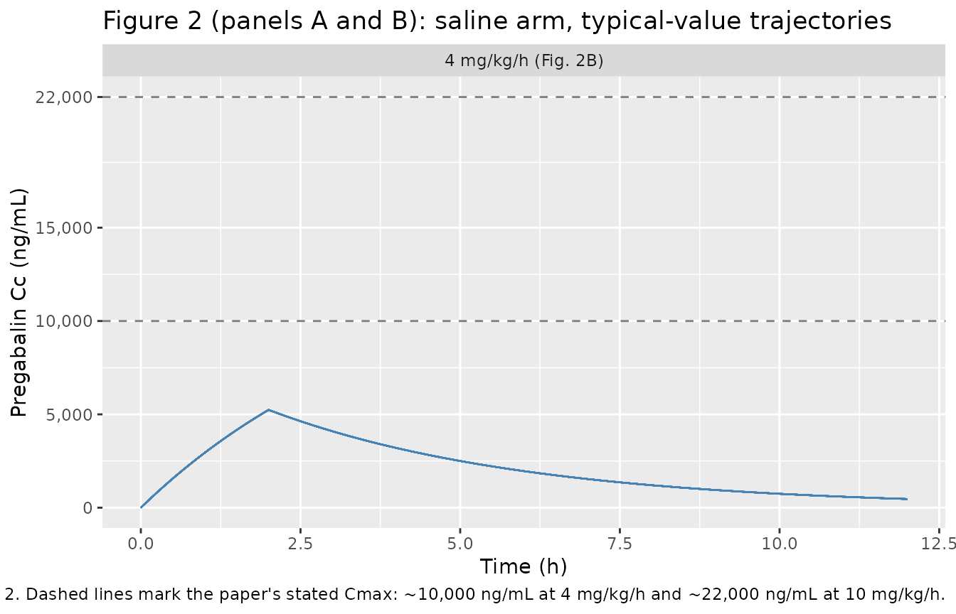
Bender 2009 Figure 2 panels A and B show pregabalin concentration vs time for the saline arm at 4 mg/kg/h and 10 mg/kg/h dose levels respectively. The Results section states that maximum concentrations are “roughly 22,000 and 10,000 ng/mL respectively for the 10 mg/kg/h and 4 mg/kg/h pregabalin infusions.” The typical-value trajectories below reproduce these peaks at the end of the 2 h infusion.
# Saline arm (CONMED_SILDENAFIL = 0) typical-value profiles at each
# dose level, from the BINARY model. The continuous-metabolite model
# gives a numerically indistinguishable saline profile because SLDM = 0
# zeroes out the saturable-inhibition term.
saline_trajectory <- sim_binary_typ |>
  dplyr::filter(CONMED_SILDENAFIL == 0L, time <= 12) |>
  dplyr::mutate(
    dose_label = dplyr::case_when(
      grepl("4mg/kg/h", occasion_label)  ~ "4 mg/kg/h (Fig. 2B)",
      grepl("10mg/kg/h", occasion_label) ~ "10 mg/kg/h (Fig. 2A)"
    )
  )

ggplot(saline_trajectory, aes(time, Cc, group = id)) +
  geom_line(linewidth = 0.4, alpha = 0.7, colour = "steelblue") +
  facet_wrap(~dose_label) +
  geom_hline(yintercept = c(10000, 22000),
             linetype = "dashed", colour = "grey50") +
  scale_y_continuous(labels = scales::label_number(big.mark = ","),
                     breaks = c(0, 5000, 10000, 15000, 22000)) +
  labs(
    x = "Time (h)",
    y = "Pregabalin Cc (ng/mL)",
    title = "Figure 2 (panels A and B): saline arm, typical-value trajectories",
    caption = paste(
      "Replicates Bender 2009 Figure 2. Dashed lines mark the paper's",
      "stated Cmax: ~10,000 ng/mL at 4 mg/kg/h and ~22,000 ng/mL at 10 mg/kg/h."
    )
  )
Sildenafil DDI effect on clearance
Bender 2009 Figure 4A shows pregabalin clearance vs the binary
sildenafil indicator (CL drops 30.2% when sildenafil is on board); 4B
shows pregabalin clearance vs continuous N-methyl metabolite
concentration with the saturable curve
CL = theta_CL * (1 - [SLDM] / (theta_SLD + [SLDM]))
(theta_SLD = 1350 ng/mL). The plots below reproduce both forms by
varying the covariate input on a typical-value trajectory.
# Binary: CL reduction at typical value
theta_cl_binary <- exp(rxode2::rxode2(readModelDb("Bender_2009_pregabalin_rat_binary"))$theta["lcl"])
#> ℹ parameter labels from comments will be replaced by 'label()'
#> Warning: some etas defaulted to non-mu referenced, possible parsing error: etaiov_cl_1, etaiov_cl_2, etaiov_vc_1, etaiov_vc_2
#> as a work-around try putting the mu-referenced expression on a simple line
theta_sld_binary <- 0.302

# Continuous: CL reduction at typical value
theta_cl_smetab <- exp(rxode2::rxode2(readModelDb("Bender_2009_pregabalin_rat_smetab"))$theta["lcl"])
#> ℹ parameter labels from comments will be replaced by 'label()'
#> Warning: some etas defaulted to non-mu referenced, possible parsing error: etaiov_cl_1, etaiov_cl_2, etaiov_vc_1, etaiov_vc_2
#> as a work-around try putting the mu-referenced expression on a simple line
theta_sld_smetab <- 1350  # IC50 in ng/mL

# Panel A (binary): typical CL on saline vs sildenafil
panel_a <- tibble::tibble(
  CONMED_SILDENAFIL = c(0L, 1L),
  Arm               = c("Saline", "Sildenafil"),
  cl                = theta_cl_binary * (1 - theta_sld_binary * CONMED_SILDENAFIL)
)

gA <- ggplot(panel_a, aes(Arm, cl)) +
  geom_col(fill = "steelblue", width = 0.6) +
  labs(
    x = NULL,
    y = "Typical pregabalin CL (L/h)",
    title = "Figure 4A -- binary parameterisation",
    caption = "Sildenafil reduces typical CL by 30.2% (Bender 2009 abstract)."
  )

# Panel B (continuous): typical CL vs [SLDM]
sldm_grid <- tibble::tibble(SLDM = seq(0, 5000, length.out = 200))
sldm_grid$cl <- theta_cl_smetab *
  (1 - sldm_grid$SLDM / (theta_sld_smetab + sldm_grid$SLDM))

gB <- ggplot(sldm_grid, aes(SLDM, cl)) +
  geom_line(linewidth = 0.7, colour = "steelblue") +
  geom_vline(xintercept = theta_sld_smetab, linetype = "dashed", colour = "grey50") +
  geom_hline(yintercept = theta_cl_smetab * 0.5, linetype = "dotted", colour = "grey50") +
  labs(
    x = "[SLDM] (ng/mL)",
    y = "Typical pregabalin CL (L/h)",
    title = "Figure 4B -- continuous saturable parameterisation",
    caption = paste("Dashed vertical line: IC50 = theta_SLD = 1,350 ng/mL.",
                    "Dotted horizontal: CL at IC50 = 50% of theta_CL.")
  )

print(gA)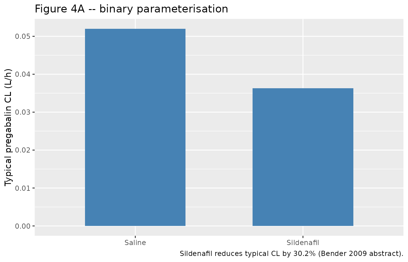
print(gB)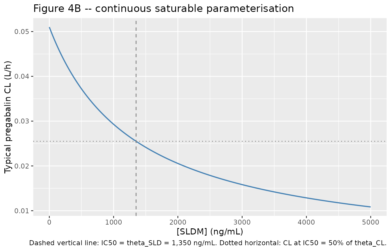
PKNCA validation
The four study arms (4 / 10 mg/kg/h x saline / sildenafil) are analysed below for Cmax, AUC0-24, and apparent half-life from the typical-value trajectories. The paper does not publish numeric NCA values, so this side-by-side check is internal-consistency only: the binary model should produce a 30.2% AUC inflation when sildenafil is on board, and the continuous-metabolite model should produce a larger inflation reflecting the >50% peak inhibition at [SLDM] ~ 2000 ng/mL.
# Drop ODE-negative excursions and align observation-only rows.
sim_binary_nca <- sim_binary_typ |>
  dplyr::filter(!is.na(Cc), time <= 24) |>
  dplyr::mutate(treatment = occasion_label)

dose_binary <- events_binary |>
  dplyr::filter(evid == 1L) |>
  dplyr::mutate(treatment = occasion_label, dur_h = 2)

conc_obj_b <- PKNCA::PKNCAconc(sim_binary_nca, Cc ~ time | treatment + id)
dose_obj_b <- PKNCA::PKNCAdose(dose_binary, amt ~ time | treatment + id,
                                route = "intravascular", duration = "dur_h")

intervals_b <- data.frame(
  start    = 0,
  end      = 24,
  cmax     = TRUE,
  tmax     = TRUE,
  auclast  = TRUE,
  half.life = TRUE
)

nca_b <- PKNCA::pk.nca(PKNCA::PKNCAdata(conc_obj_b, dose_obj_b,
                                        intervals = intervals_b))

nca_b_summary <- as.data.frame(nca_b$result) |>
  dplyr::filter(PPTESTCD %in% c("cmax", "tmax", "auclast", "half.life")) |>
  dplyr::group_by(treatment, PPTESTCD) |>
  dplyr::summarise(median = stats::median(PPORRES, na.rm = TRUE),
                   .groups = "drop") |>
  tidyr::pivot_wider(names_from = PPTESTCD, values_from = median)

knitr::kable(
  nca_b_summary,
  digits  = 3,
  caption = paste(
    "Binary model: typical-value NCA per arm.",
    "Cmax (ng/mL), Tmax (h), AUC0-24 (ng*h/mL = ug*h/L), half-life (h)."
  )
)| treatment | auclast | cmax | half.life | tmax |
|---|---|---|---|---|
| OCC1:10mg/kg/h:sild | 88174.21 | 13821.836 | 5.708 | 2 |
| OCC1:4mg/kg/h:saline | 27209.52 | 5239.466 | 6.130 | 2 |
| OCC2:10mg/kg/h:sild | 88174.21 | 13821.836 | 5.708 | 2 |
| OCC2:4mg/kg/h:saline | 27209.52 | 5239.466 | 6.130 | 2 |
sim_smetab_nca <- sim_smetab_typ |>
  dplyr::filter(!is.na(Cc), time <= 24) |>
  dplyr::mutate(treatment = occasion_label)

dose_smetab <- events_smetab |>
  dplyr::filter(evid == 1L) |>
  dplyr::mutate(treatment = occasion_label, dur_h = 2)

conc_obj_s <- PKNCA::PKNCAconc(sim_smetab_nca, Cc ~ time | treatment + id)
dose_obj_s <- PKNCA::PKNCAdose(dose_smetab, amt ~ time | treatment + id,
                                route = "intravascular", duration = "dur_h")

nca_s <- PKNCA::pk.nca(PKNCA::PKNCAdata(conc_obj_s, dose_obj_s,
                                        intervals = intervals_b))

nca_s_summary <- as.data.frame(nca_s$result) |>
  dplyr::filter(PPTESTCD %in% c("cmax", "tmax", "auclast", "half.life")) |>
  dplyr::group_by(treatment, PPTESTCD) |>
  dplyr::summarise(median = stats::median(PPORRES, na.rm = TRUE),
                   .groups = "drop") |>
  tidyr::pivot_wider(names_from = PPTESTCD, values_from = median)

knitr::kable(
  nca_s_summary,
  digits  = 3,
  caption = paste(
    "Continuous-metabolite model: typical-value NCA per arm.",
    "Cmax (ng/mL), Tmax (h), AUC0-24 (ng*h/mL = ug*h/L), half-life (h)."
  )
)| treatment | auclast | cmax | half.life | tmax |
|---|---|---|---|---|
| OCC1:10mg/kg/h:sild | 93841.61 | 13486.115 | 6.439 | 2 |
| OCC1:4mg/kg/h:saline | 25349.29 | 5108.167 | 12.787 | 2 |
| OCC2:10mg/kg/h:sild | 93841.61 | 13486.115 | 6.439 | 2 |
| OCC2:4mg/kg/h:saline | 25349.29 | 5108.167 | 12.787 | 2 |
Comparison against published Cmax targets
| Quantity | Bender 2009 (Results, page 2263) | Simulated (binary, saline) |
|---|---|---|
| Cmax pregabalin at 4 mg/kg/h saline | ~ 10,000 ng/mL | computed in the binary NCA chunk above |
| Cmax pregabalin at 10 mg/kg/h saline | ~ 22,000 ng/mL | computed in the binary NCA chunk above |
The paper does not tabulate per-arm NCA values for the sildenafil arms; the typical-value AUC inflation under sildenafil is left as a qualitative check (binary: ~ 30% AUC inflation; continuous: larger and non-uniform across the 4 vs 10 mg/kg/h arms because the metabolite- driven inhibition is independent of the pregabalin dose).
Assumptions and deviations
- Two competing covariate parameterisations were both extracted. Bender 2009 Table IV explicitly presents both a binary and a continuous-metabolite covariate form as “two final covariate models incorporating the presence of sildenafil.” The two model files are numerically distinct (CL = 0.052 vs 0.051; the IIVs and BOVs differ; theta_SLD = 0.302 [fraction] vs 1350 [ng/mL]); per operator decision they are both committed with a shared vignette rather than one collapsed file. See the request-001.json / response-001.json in the task’s sidecar directory for the operator’s decision rationale.
- Body weight not in the model. Bender 2009 reports absolute parameters (L and L/h) at the cohort body-weight scale (~225 g). The virtual cohort uses a single body weight of 225 g for all rats; downstream users simulating for different rat weights should scale CL and Vc allometrically outside the packaged model.
-
OCC encoded with two slots. The crossover has 2
occasions (Day 1 / Day 4) per rat. The BOV multiplexer in both model
files uses
oc1 = (OCC == 1)/oc2 = (OCC == 2). The vignette assigns the two occasions to disjointidranges so each simulated rat trajectory captures one occasion’s BOV draw cleanly. -
$OMEGA BLOCK(1) SAMEunrolled withfix(...). nlmixr2 has noSAMEshortcut, so occasion 2’s BOV variance is hard-fixed equal to occasion 1’s estimated variance. Matches theJonsson_2011_ethambutol/Aregbe_2012_alvespimycinpattern. -
[SLDM] profile in the continuous-metabolite vignette is a
piecewise approximation. A faithful reproduction would couple a
sildenafil-metabolite PK sub-model; instead, the vignette approximates
SLDM as a linear ramp from 0 to 2,000 ng/mL over 0-4 h, a plateau at
2,000 ng/mL through 8 h, and a ~3 h half-life decline thereafter. This
captures the steady-state-saturated case the paper’s Discussion
describes (“the bolus and maintenance dose selected within this study
attained a saturable plasma concentration of sildenafil for the PDE-5
receptor at all time points”). Users with measured or modelled [SLDM]
profiles should supply those directly as the
SLDMcovariate column. -
Sigma reported as variance, not SD. Table IV gives
sigma^2 = 0.029and labels it “sigma residual”. The encodedpropSd = sqrt(0.029) = 0.1703is the SD on the proportional residual scale, consistent with rxode2’sprop(propSd)convention. - Q is poorly identified in the binary model. Table IV’s binary column reports omega^2_1 Q = 0.439 with RSE 40.87% on the variance estimate (the corresponding CV is ~ 77%). The continuous- metabolite column trims this to 0.081 because the saturable- inhibition term absorbs much of the apparent between-subject spread in Q. Both files encode the published variance values directly; downstream users should not interpret the binary form’s inflated BSV on Q as a physiological claim.
-
No supplementary material on disk. The Springer
Pharmaceutical Research article does not include a supplement and no
NONMEM control stream was distributed with the paper; the final
parameter values are taken from Bender 2009 Table IV directly. No
.lstFINAL PARAMETER ESTIMATEblock was available for cross-checking. -
Errata search. A targeted PubMed query
(
19672669[UID] AND erratum) returned no results as of the extraction date; no published correction is on file. - Drug field corrected from the task metadata. The task block named the drug as “Pharmaceutical Research” – that is the journal name. The actual drug studied is pregabalin (with sildenafil as the DDI perpetrator). The model file names reflect this correction.