Doxycycline chicken (Petkova 2022)
Source:vignettes/articles/Petkova_2022_doxycycline_chicken.Rmd
Petkova_2022_doxycycline_chicken.RmdModel and source
- Citation: Petkova T, Yordanova A, Milanova A. Population Pharmacokinetics of Doxycycline, Administered Alone or with N-Acetylcysteine, in Chickens with Experimental Mycoplasma gallisepticum Infection. Pharmaceutics. 2022;14(11):2440. doi:10.3390/pharmaceutics14112440
- Description: Preclinical (chicken). Two-compartment population PK model with first-order absorption, absorption lag and first-order elimination, parameterised in micro-constants, for doxycycline hyclate given via drinking water at a nominal 20 mg/kg/24 h for 5 days to healthy and Mycoplasma gallisepticum-infected Ross broiler chickens with or without feed N-acetylcysteine; no covariates retained (Petkova 2022). The printed V/F and ke (CL/F = 0.728 L/kg/h) give about half of the paper’s own NCA AUC under once-daily dose records; see the vignette before using the absolute exposure scale
- Article: https://doi.org/10.3390/pharmaceutics14112440 (open access)
- Supplement (Tables S1-S4): https://www.mdpi.com/article/10.3390/pharmaceutics14112440/s1
Petkova et al. gave doxycycline hyclate to 40-day-old Ross broilers
through the drinking water at the registered dose rate of 20 mg/kg/24 h
for five days. Half of the birds had been challenged with Mycoplasma
gallisepticum at one day of age, and half of each health group also
received N-acetylcysteine (NAC, 100 mg/kg/24 h) in the feed. The authors
fitted a two-compartment model with first-order absorption, an
absorption lag and first-order elimination in Phoenix 8.3.4 (FOCE-ELS),
parameterised in micro-constants (ka, V/F,
ke, k12, k21, tlag).
Neither infection nor NAC was retained as a covariate, so the final
model has none. All parameters are apparent (oral) and per kg body
weight.
Read the Errata section before using this model for dose
prediction. The printed V/F and ke
imply an apparent clearance of 0.728 L/kg/h, which reproduces only about
half of the paper’s own observed exposure under the stated once-daily
regimen. The model is packaged exactly as printed; the vignette
quantifies the gap.
Population
Thirty-two broilers contributed to the population analysis (Section 2.2): six healthy birds on doxycycline alone (2.79 +/- 0.17 kg), six healthy birds on doxycycline + NAC (2.84 +/- 0.29 kg), ten infected birds on doxycycline alone (2.47 +/- 0.27 kg) and ten infected birds on doxycycline + NAC (2.48 +/- 0.43 kg). The medicated water was freshly prepared every 12 h and the consumed volume was recorded; the doses actually received were 24.41, 23.70, 22.18 and 23.78 mg/kg/24 h. Blood was sampled at 0.5-24 h on the first day and at 120-174 h after the start of treatment (19 samples per healthy bird, 9-10 per infected bird). Plasma doxycycline was measured by LC-MS/MS (LOQ 0.08 ug/mL); the 4.6% of samples below the LOQ were excluded from the fit. Both sexes were used; the sex mix was not reported.
The same information is available programmatically via
readModelDb("Petkova_2022_doxycycline_chicken")()$population.
Source trace
| Equation / parameter | Value | Source location |
|---|---|---|
lka (ka) |
log(0.093) 1/h | Table 1, tvka
|
lvc (V/F per kg) |
log(4.73) L/kg | Table 1, tvV/F
|
lkel (ke) |
log(0.154) 1/h | Table 1, tvke
|
lk12 (k12) |
log(4.59) 1/h | Table 1, tvk12
|
lk21 (k21) |
log(7.06) 1/h | Table 1, tvk21
|
ltlag (tlag) |
log(0.80) h | Table 1, tvtlag
|
etalka |
0.002 | Table 2, variance of eta ka |
etalvc |
0.06 | Table 2, variance of eta V |
etalkel |
1.02e-7 | Table 2, variance of eta ke |
etalk12 |
0.32 | Table 2, variance of eta k12 |
etalk21 |
0.14 | Table 2, variance of eta k21 |
etaltlag |
0.79 | Table 2, variance of eta tlag |
propSd |
0.388 | Table 1, tvCMultStdev (multiplicative residual SD) |
addSd |
0.121 ug/mL | Table 1, stdev0 (additive residual SD) |
P_i = tvP x exp(eta_i) for every parameter |
n/a | Equation 2 and the sentence after it (“The other parameters were calculated with the same algorithm”) |
| Two compartments, first-order absorption with lag, first-order elimination, micro-constant parameterisation | n/a | Section 2.6 |
Combined additive + multiplicative residual error
(combined2) |
n/a | Section 2.6 (“a multiplicative and additive error”); Table 1 footnote |
| No covariates | n/a | Section 2.6 and Results (“The tested co-variables did not improve the model and were excluded”) |
Dose in mg/kg into depot
|
n/a | Section 2.2 |
Observed data (Supplementary Tables S2 and S3)
The individual concentrations of all 32 birds are transcribed below.
A value printed with “(<LOQ)” is written here as
<value and treated as missing, as in the fit; a dash
(bird not sampled at that time) is written as ..
read_block <- function(txt, ids) {
  df <- utils::read.table(
    text = txt,
    header = FALSE,
    na.strings = ".",
    colClasses = "character"
  )
  names(df) <- c("time", paste0("chicken_", ids))
  df |>
    tidyr::pivot_longer(-time, names_to = "id", values_to = "raw") |>
    dplyr::filter(!is.na(raw)) |>
    dplyr::mutate(
      time = as.numeric(time),
      id = as.integer(sub("chicken_", "", id)),
      blq = startsWith(raw, "<"),
      conc = ifelse(blq, NA_real_, suppressWarnings(as.numeric(raw)))
    ) |>
    dplyr::select(id, time, conc, blq)
}

healthy_dox <- read_block(
  "0.5 0.253 0.171 0.213 0.133 0.224 0.282
   1 0.463 0.329 0.472 0.204 0.613 1.126
   2 0.991 0.954 1.748 0.609 1.385 1.538
   3 0.768 0.595 0.791 0.856 0.653 1.267
   4 1.083 0.570 0.907 0.697 0.670 1.659
   6 1.638 0.796 1.563 1.080 1.037 2.322
   9 1.279 1.336 1.092 1.302 1.852 2.493
   12 2.169 1.428 2.187 2.008 3.409 3.636
   14 2.419 3.053 2.018 2.142 3.287 3.357
   24 1.224 2.205 3.246 1.700 3.278 5.184
   120 1.786 1.117 2.449 1.947 2.462 2.945
   122 1.079 1.311 2.714 2.151 2.045 2.094
   124 0.941 0.994 1.294 1.112 1.135 0.825
   126 0.591 0.723 1.109 0.832 1.389 1.170
   132 0.506 0.448 0.588 0.437 0.533 0.923
   144 0.218 0.335 0.331 0.169 0.206 0.510
   152 0.123 0.150 0.218 0.107 0.115 0.247
   168 0.196 0.118 0.177 0.086 0.108 0.185
   174 0.119 0.136 0.172 0.083 <0.055 0.216",
  1:6
)

healthy_dox_nac <- read_block(
  "0.5 <0.008 <0.003 <0.002 <0.016 <0.049 0.147
   1 0.610 <0.007 <0.006 0.223 0.171 0.700
   2 1.776 <0.031 <0.036 1.814 1.001 1.561
   3 1.491 0.299 1.400 1.396 1.083 1.048
   4 2.450 1.473 2.356 1.865 1.856 1.706
   6 4.010 1.980 2.743 1.649 2.036 1.672
   9 5.007 2.779 3.710 1.873 2.830 2.345
   12 5.999 3.408 4.044 3.532 3.064 3.561
   14 5.482 3.624 3.466 2.879 3.034 3.333
   24 3.659 2.064 3.206 1.867 2.366 3.900
   120 3.107 2.763 2.892 2.025 1.946 1.481
   122 3.981 1.444 1.597 0.952 2.514 2.314
   124 2.668 0.768 1.473 0.537 1.081 1.517
   126 1.715 0.622 1.242 0.660 1.143 1.281
   132 1.004 0.341 0.920 0.416 0.917 0.671
   144 0.486 0.191 0.352 0.322 0.518 0.294
   152 0.307 0.112 0.202 0.122 0.208 0.135
   168 0.224 0.082 0.128 0.109 0.119 0.107
   174 0.209 0.096 0.124 0.127 0.142 0.114",
  7:12
)

infected_dox <- read_block(
  "0.5 <0.069 . 0.135 . 0.391 . <0.023 <0.001 . 0.092
   1 0.178 0.219 . 0.240 . <0.036 . . 0.088 0.222
   2 . 0.783 0.303 . 0.537 0.086 0.492 . 0.096 .
   3 0.489 . 0.444 0.513 . . 0.194 0.063 . 0.163
   4 . 0.876 . 1.140 1.184 . . 0.150 0.505 0.400
   6 1.030 1.020 1.047 . 1.619 1.259 . . 1.489 .
   9 1.544 . . 1.458 . 1.797 2.476 1.137 . 1.200
   12 . 1.299 1.836 . 2.685 . 3.037 . 2.098 2.574
   14 . 1.675 2.249 2.125 . 1.733 . 1.804 2.553 .
   24 1.654 . . 2.640 4.147 . 2.751 1.588 . 2.597
   120 . 1.501 3.304 . 2.078 2.805 2.089 . 2.356 .
   122 2.609 . 2.872 2.837 . 2.504 . 1.477 . 2.294
   124 1.586 1.095 . 1.820 1.327 . 1.768 . 2.012 .
   126 . 0.913 1.080 . . 1.298 . 0.999 0.887 0.563
   132 0.637 . 0.522 . 0.624 . 0.799 0.298 . 0.481
   144 . 0.273 . 0.286 0.328 0.445 0.461 . 0.466 .
   152 0.211 0.166 0.183 . . 0.132 . 0.211 . 0.124
   168 0.239 . 0.161 0.193 0.356 . 0.283 . 0.376 .
   174 . 0.158 . 0.161 . 0.110 . 0.166 0.232 0.114",
  13:22
)

infected_dox_nac <- read_block(
  "0.5 <0.003 . <0.032 . <0.014 . 0.196 0.294 . <0.003
   1 0.727 0.378 . <0.020 . 0.305 . . <0.038 <0.008
   2 . 1.524 0.353 . 0.224 0.938 0.674 . 0.249 .
   3 1.172 . 0.463 0.434 . . 0.759 0.552 . 0.137
   4 . 2.040 . 1.198 1.254 . . 0.762 0.301 0.631
   6 1.653 1.836 0.910 . 1.312 0.960 . . 0.775 .
   9 1.430 . . 1.995 . 1.750 2.587 1.533 . 1.644
   12 . 1.918 1.152 . 1.991 . 4.410 . 1.723 2.044
   14 . 6.907 2.050 2.670 . 1.104 . 2.000 2.159 .
   24 1.824 . . 2.680 1.271 . 4.136 2.495 . 2.412
   120 . 4.087 2.098 . 1.748 2.976 2.236 . 2.100 .
   122 1.549 . 1.717 2.914 . 2.734 . 2.486 . 2.331
   124 1.359 1.219 . 2.418 0.995 . 2.223 . 1.388 .
   126 . 0.799 0.470 . . 0.883 . 2.102 0.765 0.833
   132 0.562 . 0.263 . 0.315 . 0.419 0.565 . 0.420
   144 . 0.557 . 0.231 0.197 0.246 0.293 . 0.231 .
   152 0.272 0.420 0.181 . . 0.178 . 0.174 . 0.134
   168 0.218 . 0.177 0.189 0.137 . 0.159 . 0.179 .
   174 . 0.181 . 0.127 . 0.111 . 0.141 0.138 0.116",
  23:32
)

groups <- tibble::tibble(
  group = factor(
    c(
      "Healthy, doxycycline",
      "Healthy, doxycycline + NAC",
      "Infected, doxycycline",
      "Infected, doxycycline + NAC"
    ),
    levels = c(
      "Healthy, doxycycline",
      "Healthy, doxycycline + NAC",
      "Infected, doxycycline",
      "Infected, doxycycline + NAC"
    )
  ),
  # Section 2.2: doses actually received (mg/kg per 24 h)
  daily_dose = c(24.41, 23.70, 22.18, 23.78)
)

observed <- dplyr::bind_rows(
  dplyr::mutate(healthy_dox, group = groups$group[1]),
  dplyr::mutate(healthy_dox_nac, group = groups$group[2]),
  dplyr::mutate(infected_dox, group = groups$group[3]),
  dplyr::mutate(infected_dox_nac, group = groups$group[4])
)

observed |>
  dplyr::group_by(group) |>
  dplyr::summarise(
    birds = dplyr::n_distinct(id),
    samples = dplyr::n(),
    below_loq = sum(blq)
  ) |>
knitr::kable(caption = "Transcribed Supplementary Tables S2 and S3.")| group | birds | samples | below_loq |
|---|---|---|---|
| Healthy, doxycycline | 6 | 114 | 1 |
| Healthy, doxycycline + NAC | 6 | 114 | 9 |
| Infected, doxycycline | 10 | 114 | 4 |
| Infected, doxycycline + NAC | 10 | 114 | 7 |
stopifnot(
  dplyr::n_distinct(observed$id) == 32,
  sum(observed$blq) == 21
)
How the dose was recorded
Doxycycline was taken up with the drinking water, and the water was freshly prepared every 12 h. The paper states the regimen as 20 mg/kg/24 h and gives the actually received daily doses, but does not say how the intake was entered as dose records in the Phoenix data set. The simulations below therefore carry two readings side by side:
- Stated regimen (q24). The group’s received daily dose as an oral bolus every 24 h, five doses (0-96 h). This is the regimen the paper describes.
- Daily dose at each water refresh (q12). The same daily dose entered at every 12-h water refresh, ten doses (0-108 h). This doubles the total amount and is not a regimen the paper describes. It is included only because it is the reading under which the printed parameters reproduce the paper’s own exposure (see Errata).
make_events <- function(daily_dose, reading, ids, obs_times) {
  if (reading == "Stated regimen (q24)") {
    dose_times <- seq(0, 96, by = 24)
  } else {
    dose_times <- seq(0, 108, by = 12)
  }
  doses <- tidyr::expand_grid(id = ids, time = dose_times) |>
    dplyr::mutate(amt = daily_dose, evid = 1L, cmt = "depot")
  obs <- tidyr::expand_grid(id = ids, time = obs_times) |>
    dplyr::mutate(amt = 0, evid = 0L, cmt = "central")
  dplyr::bind_rows(doses, obs) |>
    dplyr::arrange(id, time, dplyr::desc(evid)) |>
    as.data.frame()
}
readings <- c("Stated regimen (q24)", "Daily dose at each water refresh (q12)")
study_times <- c(
  0, 0.5, 1, 2, 3, 4, 6, 9, 12, 14, 24,
  120, 122, 124, 126, 132, 144, 152, 168, 174
)
Typical-value exposure against the paper’s NCA
For a linear model, the area under the whole concentration-time curve
equals the total absorbed dose divided by the apparent clearance,
AUC0-inf = n_doses x D / (V/F x ke), whatever the dosing
times. With the printed V/F = 4.73 L/kg and ke
= 0.154 1/h, CL/F = 0.728 L/kg/h. The table compares that
closed form, and the numerically integrated typical-value profile, with
the geometric-mean AUC0-inf of Supplementary Table S4.
mod <- readModelDb("Petkova_2022_doxycycline_chicken")
mod_typical <- rxode2::zeroRe(mod)
#> ℹ parameter labels from comments will be replaced by 'label()'

cl_f <- 4.73 * 0.154
dense_times <- sort(unique(c(seq(0, 200, by = 0.05), seq(200, 600, by = 1))))

typical_auc <- tidyr::expand_grid(groups, reading = readings) |>
  dplyr::rowwise() |>
  dplyr::mutate(
    n_doses = ifelse(reading == readings[1], 5, 10),
    closed_form = n_doses * daily_dose / cl_f,
    numeric = {
      ev <- make_events(daily_dose, reading, 1L, dense_times)
      s <- as.data.frame(rxode2::rxSolve(mod_typical, events = ev))
      sum(diff(s$time) * (head(s$Cc, -1) + tail(s$Cc, -1)) / 2)
    }
  ) |>
  dplyr::ungroup()
#> ℹ omega/sigma items treated as zero: 'etalka', 'etalvc', 'etalkel', 'etalk12', 'etalk21', 'etaltlag'
#> ℹ omega/sigma items treated as zero: 'etalka', 'etalvc', 'etalkel', 'etalk12', 'etalk21', 'etaltlag'
#> ℹ omega/sigma items treated as zero: 'etalka', 'etalvc', 'etalkel', 'etalk12', 'etalk21', 'etaltlag'
#> ℹ omega/sigma items treated as zero: 'etalka', 'etalvc', 'etalkel', 'etalk12', 'etalk21', 'etaltlag'
#> ℹ omega/sigma items treated as zero: 'etalka', 'etalvc', 'etalkel', 'etalk12', 'etalk21', 'etaltlag'
#> ℹ omega/sigma items treated as zero: 'etalka', 'etalvc', 'etalkel', 'etalk12', 'etalk21', 'etaltlag'
#> ℹ omega/sigma items treated as zero: 'etalka', 'etalvc', 'etalkel', 'etalk12', 'etalk21', 'etaltlag'
#> ℹ omega/sigma items treated as zero: 'etalka', 'etalvc', 'etalkel', 'etalk12', 'etalk21', 'etaltlag'

# Table S4, AUC0-inf geometric means (h*ug/mL)
table_s4 <- tibble::tibble(
  group = groups$group,
  cmax = c(3.11, 3.93, 2.32, 2.59),
  tmax = c(16.33, 13.82, 16.36, 16.11),
  aucinf.obs = c(293.21, 339.38, 288.19, 303.89)
)

typical_auc <- typical_auc |>
  dplyr::left_join(table_s4, by = "group") |>
  dplyr::mutate(ratio = closed_form / aucinf.obs)

typical_auc |>
  dplyr::select(group, reading, closed_form, numeric, aucinf.obs, ratio) |>
  dplyr::rename(
    Group = group,
    `Dose records` = reading,
    `Model AUC0-inf, closed form` = closed_form,
    `Model AUC0-inf, integrated` = numeric,
    `Table S4 AUC0-inf` = aucinf.obs,
    `Model / Table S4` = ratio
  ) |>
  knitr::kable(
    digits = c(0, 0, 1, 1, 1, 2),
    caption = "Typical-value AUC0-inf (h*ug/mL) under the two dose readings."
)| Group | Dose records | Model AUC0-inf, closed form | Model AUC0-inf, integrated | Table S4 AUC0-inf | Model / Table S4 |
|---|---|---|---|---|---|
| Healthy, doxycycline | Stated regimen (q24) | 167.6 | 167.6 | 293.2 | 0.57 |
| Healthy, doxycycline | Daily dose at each water refresh (q12) | 335.1 | 335.1 | 293.2 | 1.14 |
| Healthy, doxycycline + NAC | Stated regimen (q24) | 162.7 | 162.7 | 339.4 | 0.48 |
| Healthy, doxycycline + NAC | Daily dose at each water refresh (q12) | 325.4 | 325.4 | 339.4 | 0.96 |
| Infected, doxycycline | Stated regimen (q24) | 152.2 | 152.2 | 288.2 | 0.53 |
| Infected, doxycycline | Daily dose at each water refresh (q12) | 304.5 | 304.5 | 288.2 | 1.06 |
| Infected, doxycycline + NAC | Stated regimen (q24) | 163.2 | 163.2 | 303.9 | 0.54 |
| Infected, doxycycline + NAC | Daily dose at each water refresh (q12) | 326.5 | 326.5 | 303.9 | 1.07 |
stopifnot(
  # The integrated profile is the same parameters as the closed form; any gap
  # is pure numerical error (truncation at 600 h and the trapezoid).
  all(abs(typical_auc$numeric / typical_auc$closed_form - 1) < 0.01),
  # Stated regimen: the printed parameters give about half the observed AUC.
  all(typical_auc$ratio[typical_auc$reading == readings[1]] > 0.45),
  all(typical_auc$ratio[typical_auc$reading == readings[1]] < 0.60),
  # Daily dose at each refresh: within about 15% of every group.
  all(typical_auc$ratio[typical_auc$reading == readings[2]] > 0.90),
  all(typical_auc$ratio[typical_auc$reading == readings[2]] < 1.20)
)
Under the stated regimen the printed parameters give 48-57% of the observed AUC0-inf. Entering the daily dose at every water refresh gives 96-114%.
Typical-value profiles against the observed data
typical_profiles <- tidyr::expand_grid(groups, reading = readings) |>
  dplyr::rowwise() |>
  dplyr::reframe({
    ev <- make_events(daily_dose, reading, 1L, seq(0, 180, by = 0.25))
    s <- as.data.frame(rxode2::rxSolve(mod_typical, events = ev))
    tibble::tibble(group = group, reading = reading, time = s$time, Cc = s$Cc)
  })
#> ℹ omega/sigma items treated as zero: 'etalka', 'etalvc', 'etalkel', 'etalk12', 'etalk21', 'etaltlag'
#> ℹ omega/sigma items treated as zero: 'etalka', 'etalvc', 'etalkel', 'etalk12', 'etalk21', 'etaltlag'
#> ℹ omega/sigma items treated as zero: 'etalka', 'etalvc', 'etalkel', 'etalk12', 'etalk21', 'etaltlag'
#> ℹ omega/sigma items treated as zero: 'etalka', 'etalvc', 'etalkel', 'etalk12', 'etalk21', 'etaltlag'
#> ℹ omega/sigma items treated as zero: 'etalka', 'etalvc', 'etalkel', 'etalk12', 'etalk21', 'etaltlag'
#> ℹ omega/sigma items treated as zero: 'etalka', 'etalvc', 'etalkel', 'etalk12', 'etalk21', 'etaltlag'
#> ℹ omega/sigma items treated as zero: 'etalka', 'etalvc', 'etalkel', 'etalk12', 'etalk21', 'etaltlag'
#> ℹ omega/sigma items treated as zero: 'etalka', 'etalvc', 'etalkel', 'etalk12', 'etalk21', 'etaltlag'

ggplot() +
  geom_point(
    data = dplyr::filter(observed, !blq),
    aes(time, conc),
    colour = "grey40",
    size = 1
  ) +
  geom_line(
    data = typical_profiles,
    aes(time, Cc, colour = reading),
    linewidth = 0.7
  ) +
  facet_wrap(~group) +
  labs(
    x = "Time after the start of treatment (h)",
    y = "Doxycycline plasma concentration (ug/mL)",
    colour = "Dose records"
  ) +
  theme_bw() +
  theme(legend.position = "bottom")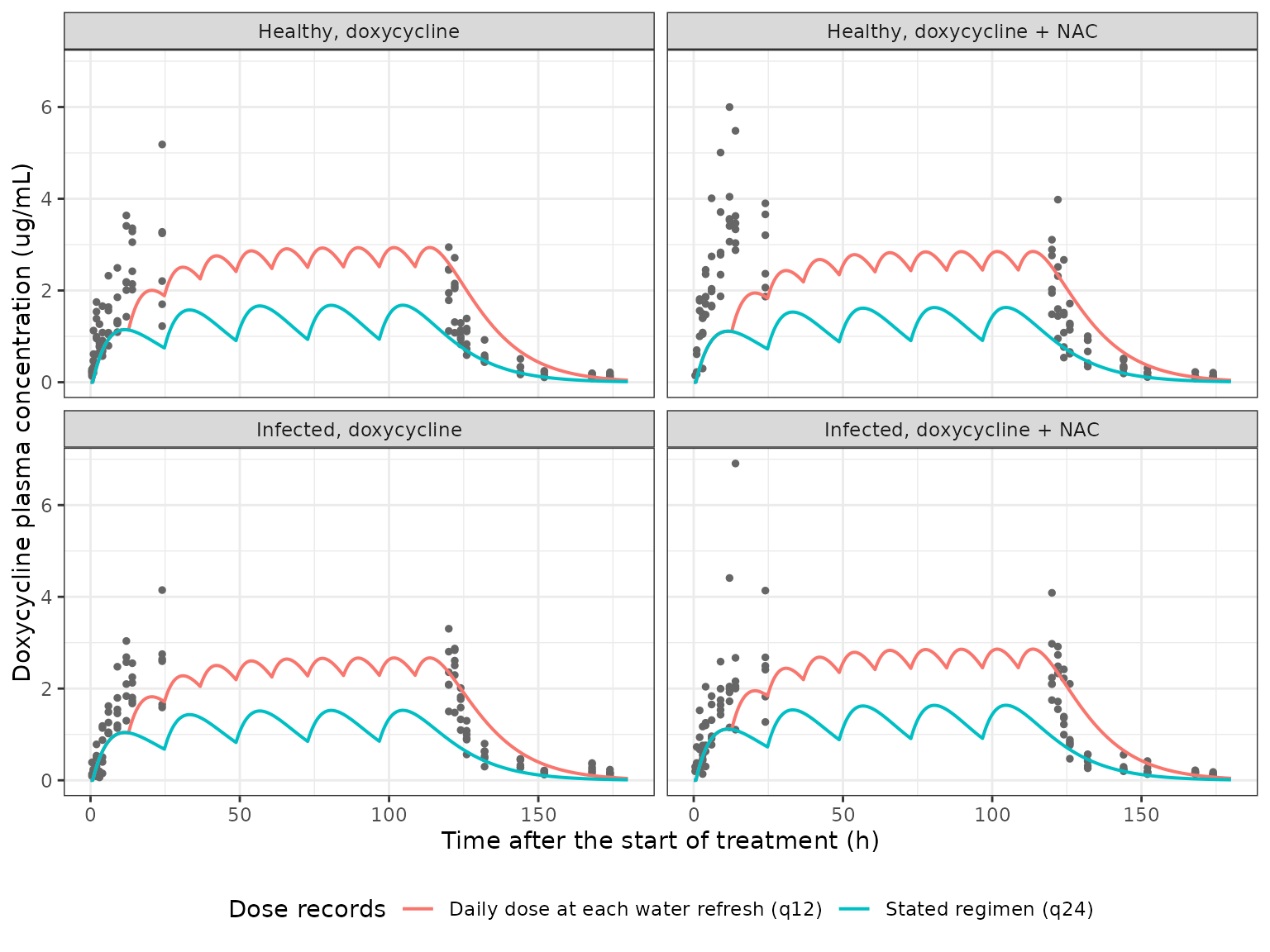
The observed concentrations rise to about 2-3 ug/mL by 12-24 h and are still about 2 ug/mL at the end of treatment (120 h). The typical profile under the stated regimen peaks near 1 ug/mL after each dose; the daily-dose-every-12-h reading roughly doubles it, to about the observed level.
Visual predictive check
Figure 1b of the paper is a VPC of the pooled data (observed and predicted 10th, 50th and 90th percentiles). The simulation below gives 50 virtual birds per group (200 per reading) the group’s received dose under each reading, with the full IIV and residual error, and compares the simulated percentiles with the percentiles of the observed data at each sampling time.
rxode2::rxSetSeed(20221111)
n_per_group <- 50

vpc_sim <- tidyr::expand_grid(groups, reading = readings) |>
  dplyr::mutate(row = dplyr::row_number()) |>
  dplyr::rowwise() |>
  dplyr::reframe({
    ids <- (row - 1) * n_per_group + seq_len(n_per_group)
    ev <- make_events(daily_dose, reading, ids, study_times[-1])
    s <- as.data.frame(rxode2::rxSolve(mod, events = ev))
    tibble::tibble(
      group = group,
      reading = reading,
      id = as.integer(as.character(s$id)),
      time = s$time,
      Cc = s$Cc,
      sim = s$sim
    )
  })
#> ℹ parameter labels from comments will be replaced by 'label()'

pctl <- function(x, p) as.numeric(stats::quantile(x, p, na.rm = TRUE))
vpc_sim_summary <- vpc_sim |>
  dplyr::group_by(reading, time) |>
  dplyr::summarise(
    p10 = pctl(sim, 0.1),
    p50 = pctl(sim, 0.5),
    p90 = pctl(sim, 0.9),
    .groups = "drop"
  )
vpc_obs_summary <- observed |>
  dplyr::filter(!blq) |>
  dplyr::group_by(time) |>
  dplyr::summarise(
    p10 = pctl(conc, 0.1),
    p50 = pctl(conc, 0.5),
    p90 = pctl(conc, 0.9),
    .groups = "drop"
  )

ggplot(vpc_sim_summary, aes(time)) +
  geom_ribbon(aes(ymin = p10, ymax = p90), fill = "steelblue", alpha = 0.25) +
  geom_line(aes(y = p50), colour = "steelblue") +
  geom_point(data = vpc_obs_summary, aes(y = p50), colour = "black") +
  geom_point(
    data = vpc_obs_summary,
    aes(y = p10),
    colour = "black",
    shape = 2,
    size = 1
  ) +
  geom_point(
    data = vpc_obs_summary,
    aes(y = p90),
    colour = "black",
    shape = 6,
    size = 1
  ) +
  facet_wrap(~reading) +
  labs(
    x = "Time after the start of treatment (h)",
    y = "Doxycycline plasma concentration (ug/mL)",
    caption = paste(
      "Shaded: simulated 10th-90th percentiles; line: simulated median.",
      "Points: observed 10th, 50th and 90th percentiles (Tables S2 and S3)."
    )
  ) +
  theme_bw()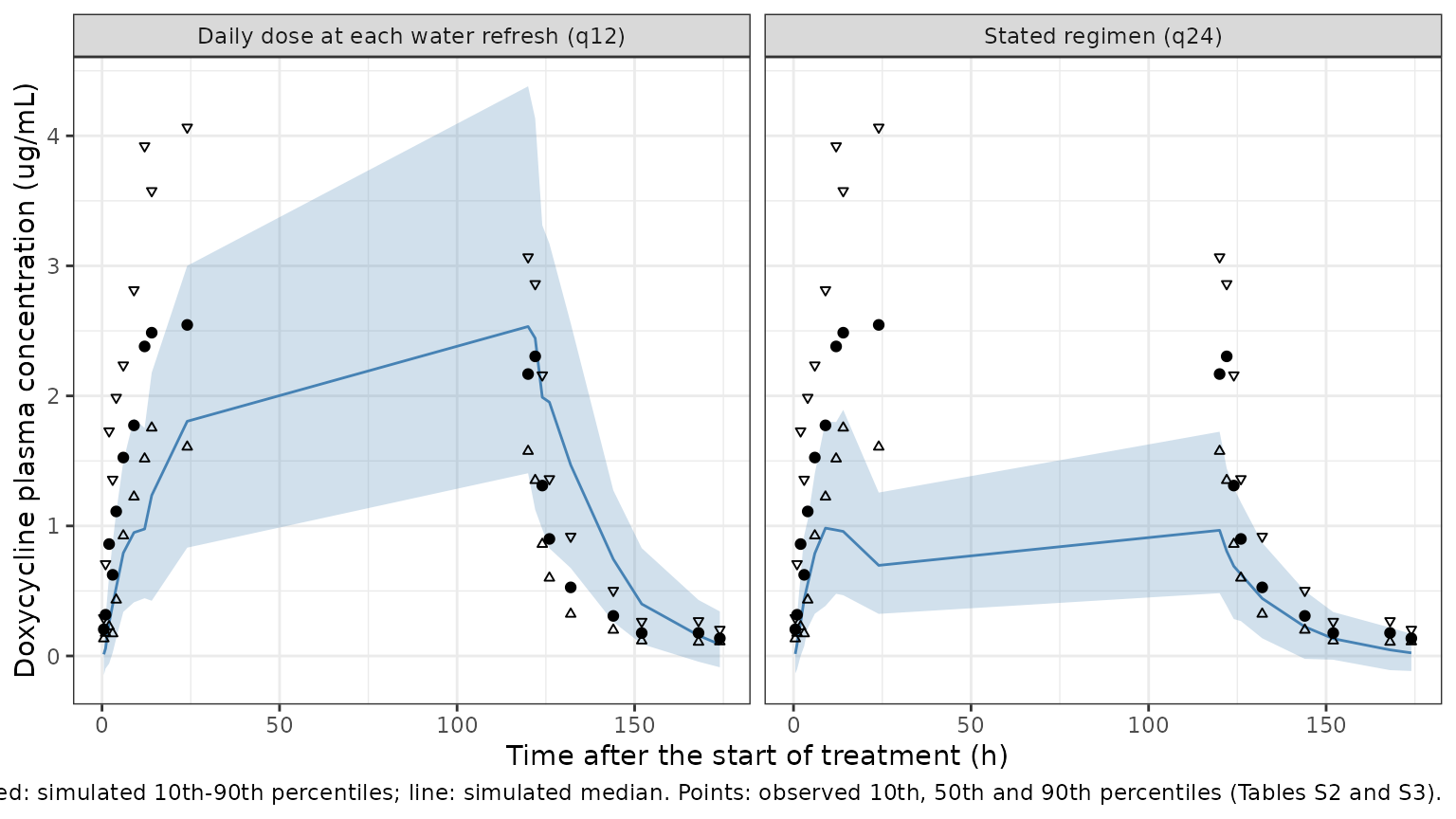
Replicates Figure 1b of Petkova 2022. The paper’s own VPC shows a predicted median near 2 ug/mL through 24-120 h, in line with the observed data. Under the stated regimen the packaged parameters give well under that level. The daily-dose-every-12-h reading comes closer, particularly at the end of treatment, but still sits below the observed medians on the first day, when only one or two refresh doses have been given.
vpc_check <- vpc_sim_summary |>
  dplyr::inner_join(vpc_obs_summary, by = "time", suffix = c("_sim", "_obs")) |>
  dplyr::mutate(
    window = dplyr::case_when(
      time >= 12 & time <= 24 ~ "Day 1 (12-24 h)",
      time >= 120 & time <= 124 ~ "End of treatment (120-124 h)"
    )
  ) |>
  dplyr::filter(!is.na(window)) |>
  dplyr::group_by(reading, window) |>
  dplyr::summarise(
    median_ratio = stats::median(p50_sim / p50_obs),
    .groups = "drop"
  )
vpc_check |>
  dplyr::rename(
    `Dose records` = reading,
    Window = window,
    `Simulated / observed median` = median_ratio
  ) |>
  knitr::kable(
    digits = 2,
    caption = "Ratio of simulated to observed median concentration, median over the sampling times in each window."
)| Dose records | Window | Simulated / observed median |
|---|---|---|
| Daily dose at each water refresh (q12) | Day 1 (12-24 h) | 0.50 |
| Daily dose at each water refresh (q12) | End of treatment (120-124 h) | 1.17 |
| Stated regimen (q24) | Day 1 (12-24 h) | 0.39 |
| Stated regimen (q24) | End of treatment (120-124 h) | 0.45 |
ratio_q24 <- stats::median(vpc_check$median_ratio[vpc_check$reading == readings[1]])
ratio_q12 <- stats::median(vpc_check$median_ratio[vpc_check$reading == readings[2]])
stopifnot(
  # Stated regimen: well under half to two-thirds of the observed level.
  ratio_q24 < 0.65,
  # The doubled-dose reading roughly doubles the level (linear model).
  ratio_q12 / ratio_q24 > 1.5
)
NCA against Supplementary Table S4
The paper’s NCA (Phoenix, Section 2.5) used the study sampling times. The individual predictions of the same 50 virtual birds per group are summarised with PKNCA on the study grid (time zero added), with AUC0-inf computed over the whole profile and extrapolated from the terminal phase after the last sample at 174 h.
nca_conc <- dplyr::select(vpc_sim, reading, group, id, time, Cc)

nca_conc <- dplyr::bind_rows(
  nca_conc,
  dplyr::distinct(nca_conc, reading, group, id) |>
    dplyr::mutate(time = 0, Cc = 0)
) |>
  dplyr::filter(!is.na(Cc)) |>
  dplyr::mutate(treatment = paste(reading, group, sep = " | ")) |>
  dplyr::arrange(treatment, id, time)

nca_dose <- dplyr::distinct(nca_conc, reading, group, treatment, id) |>
  dplyr::left_join(groups, by = "group") |>
  dplyr::mutate(time = 0, amt = daily_dose)

conc_obj <- PKNCA::PKNCAconc(nca_conc, Cc ~ time | treatment + id)
dose_obj <- PKNCA::PKNCAdose(nca_dose, amt ~ time | treatment + id)
intervals <- data.frame(
  start = 0,
  end = Inf,
  cmax = TRUE,
  tmax = TRUE,
  aucinf.obs = TRUE
)
nca_res <- PKNCA::pk.nca(PKNCA::PKNCAdata(conc_obj, dose_obj, intervals = intervals))

reference <- tidyr::expand_grid(reading = readings, table_s4) |>
  dplyr::mutate(treatment = paste(reading, group, sep = " | ")) |>
  dplyr::select(treatment, cmax, tmax, aucinf.obs)

nca_table <- ncaComparisonTable(
  nca_res,
  reference,
  by = "treatment",
  units = c(cmax = "ug/mL", tmax = "h", aucinf.obs = "h*ug/mL")
)
nca_table |>
  dplyr::rename(`Dose records | group` = treatment) |>
  knitr::kable(
    caption = paste(
      "Simulated (median of 50 virtual birds per group) versus Table S4",
      "(geometric mean) NCA."
    )
)| NCA parameter | Dose records | group | Reference | Simulated | % diff |
|---|---|---|---|---|
| Cmax (ug/mL) | Stated regimen (q24) | Healthy, doxycycline | 3.11 | 1.13 | -63.6%* |
| Cmax (ug/mL) | Stated regimen (q24) | Healthy, doxycycline + NAC | 3.93 | 1.19 | -69.7%* |
| Cmax (ug/mL) | Stated regimen (q24) | Infected, doxycycline | 2.32 | 1.02 | -56.2%* |
| Cmax (ug/mL) | Stated regimen (q24) | Infected, doxycycline + NAC | 2.59 | 1.04 | -60.0%* |
| Cmax (ug/mL) | Daily dose at each water refresh (q12) | Healthy, doxycycline | 3.11 | 2.51 | -19.4% |
| Cmax (ug/mL) | Daily dose at each water refresh (q12) | Healthy, doxycycline + NAC | 3.93 | 2.67 | -32.0%* |
| Cmax (ug/mL) | Daily dose at each water refresh (q12) | Infected, doxycycline | 2.32 | 2.48 | +6.8% |
| Cmax (ug/mL) | Daily dose at each water refresh (q12) | Infected, doxycycline + NAC | 2.59 | 2.71 | +4.5% |
| Tmax (h) | Stated regimen (q24) | Healthy, doxycycline | 16.3 | 12 | -26.5%* |
| Tmax (h) | Stated regimen (q24) | Healthy, doxycycline + NAC | 13.8 | 12 | -13.2% |
| Tmax (h) | Stated regimen (q24) | Infected, doxycycline | 16.4 | 12 | -26.7%* |
| Tmax (h) | Stated regimen (q24) | Infected, doxycycline + NAC | 16.1 | 12 | -25.5%* |
| Tmax (h) | Daily dose at each water refresh (q12) | Healthy, doxycycline | 16.3 | 120 | +634.8%* |
| Tmax (h) | Daily dose at each water refresh (q12) | Healthy, doxycycline + NAC | 13.8 | 120 | +768.3%* |
| Tmax (h) | Daily dose at each water refresh (q12) | Infected, doxycycline | 16.4 | 120 | +633.5%* |
| Tmax (h) | Daily dose at each water refresh (q12) | Infected, doxycycline + NAC | 16.1 | 120 | +644.9%* |
| AUC0-∞ (obs) (h*ug/mL) | Stated regimen (q24) | Healthy, doxycycline | 293 | 115 | -60.9%* |
| AUC0-∞ (obs) (h*ug/mL) | Stated regimen (q24) | Healthy, doxycycline + NAC | 339 | 126 | -62.8%* |
| AUC0-∞ (obs) (h*ug/mL) | Stated regimen (q24) | Infected, doxycycline | 288 | 104 | -63.9%* |
| AUC0-∞ (obs) (h*ug/mL) | Stated regimen (q24) | Infected, doxycycline + NAC | 304 | 108 | -64.4%* |
| AUC0-∞ (obs) (h*ug/mL) | Daily dose at each water refresh (q12) | Healthy, doxycycline | 293 | 283 | -3.3% |
| AUC0-∞ (obs) (h*ug/mL) | Daily dose at each water refresh (q12) | Healthy, doxycycline + NAC | 339 | 299 | -11.9% |
| AUC0-∞ (obs) (h*ug/mL) | Daily dose at each water refresh (q12) | Infected, doxycycline | 288 | 276 | -4.3% |
| AUC0-∞ (obs) (h*ug/mL) | Daily dose at each water refresh (q12) | Infected, doxycycline + NAC | 304 | 301 | -1.0% |
- differs from reference by more than ±20%.
nca_auc <- as.data.frame(nca_res) |>
  dplyr::filter(PPTESTCD == "aucinf.obs") |>
  dplyr::group_by(treatment) |>
  dplyr::summarise(sim = stats::median(PPORRES)) |>
  dplyr::left_join(reference, by = "treatment") |>
  dplyr::mutate(
    reading = sub(" \\| .*$", "", treatment),
    ratio = sim / aucinf.obs
  )
stopifnot(
  # A transcription or unit error would move these by tens of percent.
  stats::median(nca_auc$ratio[nca_auc$reading == readings[1]]) < 0.70,
  abs(stats::median(nca_auc$ratio[nca_auc$reading == readings[2]]) - 1) < 0.25
)
The observed Tmax of 14-16 h is an artefact of the sampling design: no sample was taken between 24 and 120 h, so the observed peak is the highest of the first-day samples. Under the stated regimen the simulated Tmax on the same grid behaves the same way (12 h, just before the 24-h dose). Under the daily-dose-every-12-h reading the last dose is at 108 h, so the 120-h sample is the highest and the simulated Tmax is 120 h; the Tmax rows for that reading reflect the dose timing, not the parameters. Under the stated regimen the simulated Cmax and AUC0-inf are about 35-45% of the Table S4 values (the sparse 24-120 h gap also loses part of the inter-dose peaks that the closed-form AUC above includes); under the daily-dose-every-12-h reading AUC0-inf agrees within about 15% and Cmax within about 30%.
Probability of target attainment (Table 3)
Section 2.7 simulated 5000 birds for 24 h at 1.5-h increments and
computed the percentage of the 24-h dosing interval with unbound
concentration above the MIC, with the unbound fraction fixed at 0.5. The
chunk below repeats that on 200 virtual birds for the first 24 h after a
20 mg/kg dose, under both readings, and also evaluates the paper’s
Equation 5,
%T>MIC = ln(Dose x f / (V x MIC)) / ke x 100 / tau, at
the typical values.
rxode2::rxSetSeed(2440)
pta_times <- seq(0, 24, by = 1.5)
pta_sim <- dplyr::bind_rows(lapply(readings, function(r) {
  dose_times <- if (r == readings[1]) 0 else c(0, 12)
  ev <- dplyr::bind_rows(
    tidyr::expand_grid(id = 1:200, time = dose_times) |>
      dplyr::mutate(amt = 20, evid = 1L, cmt = "depot"),
    tidyr::expand_grid(id = 1:200, time = pta_times) |>
      dplyr::mutate(amt = 0, evid = 0L, cmt = "central")
  ) |>
    dplyr::arrange(id, time, dplyr::desc(evid)) |>
    as.data.frame()
  s <- as.data.frame(rxode2::rxSolve(mod, events = ev))
  tibble::tibble(reading = r, id = s$id, time = s$time, Cc = s$Cc)
}))

mics <- c(0.25, 0.5, 1, 2)
quantile_probs <- c(0.95, 0.90, 0.75, 0.50, 0.25, 0.10, 0.05)
pta_ft <- function(r, m) {
  ft <- pta_sim |>
    dplyr::filter(reading == r, time < 24) |>
    dplyr::group_by(id) |>
    dplyr::summarise(ft = 100 * mean(0.5 * Cc > m))
  tibble::tibble(
    reading = r,
    mic = m,
    quantile = paste0(100 * (1 - quantile_probs), "%"),
    ft = as.numeric(stats::quantile(ft$ft, quantile_probs))
  )
}
pta_grid <- tidyr::expand_grid(reading = readings, mic = mics)
pta_model <- dplyr::bind_rows(
  mapply(pta_ft, pta_grid$reading, pta_grid$mic, SIMPLIFY = FALSE)
)

# Table 3 of Petkova 2022 (columns are the 5th..95th percentiles)
table3 <- tibble::tibble(
  mic = rep(mics, each = 7),
  quantile = rep(paste0(c(5, 10, 25, 50, 75, 90, 95), "%"), 4),
  ft = c(
    100, 100, 100, 100, 100, 100, 100,
    100, 100, 100, 100, 92.65, 79.60, 72.46,
    100, 91.89, 76.23, 62.07, 49.61, 40.23, 35.39,
    44.74, 38.05, 27.66, 17.50, 9.45, 4.35, 2.21
  )
)

pta_wide <- dplyr::bind_rows(
  dplyr::mutate(table3, source = "Table 3"),
  dplyr::mutate(pta_model, source = reading) |> dplyr::select(-reading)
) |>
  dplyr::filter(quantile %in% c("10%", "50%", "90%")) |>
  tidyr::pivot_wider(names_from = quantile, values_from = ft) |>
  dplyr::arrange(mic, source)
pta_wide |>
  dplyr::rename(`MIC (mg/L)` = mic, Source = source) |>
  knitr::kable(
    digits = c(2, 0, 1, 1, 1),
    caption = "%fT>MIC over the first 24 h: Table 3 versus the packaged model (10th, 50th and 90th percentile of birds)."
)| MIC (mg/L) | Source | 10% | 50% | 90% |
|---|---|---|---|---|
| 0.25 | Daily dose at each water refresh (q12) | 87.5 | 81.2 | 62.5 |
| 0.25 | Stated regimen (q24) | 87.5 | 81.2 | 56.2 |
| 0.25 | Table 3 | 100.0 | 100.0 | 100.0 |
| 0.50 | Daily dose at each water refresh (q12) | 75.0 | 43.8 | 25.0 |
| 0.50 | Stated regimen (q24) | 63.1 | 0.0 | 0.0 |
| 0.50 | Table 3 | 100.0 | 100.0 | 79.6 |
| 1.00 | Daily dose at each water refresh (q12) | 25.6 | 0.0 | 0.0 |
| 1.00 | Stated regimen (q24) | 0.0 | 0.0 | 0.0 |
| 1.00 | Table 3 | 91.9 | 62.1 | 40.2 |
| 2.00 | Daily dose at each water refresh (q12) | 0.0 | 0.0 | 0.0 |
| 2.00 | Stated regimen (q24) | 0.0 | 0.0 | 0.0 |
| 2.00 | Table 3 | 38.0 | 17.5 | 4.3 |
eq5 <- tibble::tibble(
  `MIC (mg/L)` = mics,
  `Equation 5 at typical values (%)` = pmin(
    100,
    pmax(0, log(20 * 0.5 / (4.73 * mics)) / 0.154 * 100 / 24)
  )
)
knitr::kable(eq5, digits = c(2, 1), caption = "Paper Equation 5 at the typical V/F and ke.")| MIC (mg/L) | Equation 5 at typical values (%) |
|---|---|
| 0.25 | 57.8 |
| 0.50 | 39.0 |
| 1.00 | 20.3 |
| 2.00 | 1.5 |
Table 3 cannot be reproduced from the printed parameters under either reading or from Equation 5. Table 3 has 5% of birds above 2 ug/mL unbound (4 ug/mL total) for 45% of the day, whereas the typical total concentration under the stated regimen does not reach 1.5 ug/mL in the first 24 h. The table is shown for completeness only.
Assumptions and deviations
-
Dosing as oral boluses. The drug was taken up with
the drinking water across the day. The paper does not describe the dose
records of its data set; the simulations enter each daily (or
per-refresh) amount as an oral bolus into
depot, which the absorption lag and slowka(0.093 1/h) smooth into a near-continuous input. - Received doses. The simulations use each group’s actually received dose (Section 2.2: 24.41, 23.70, 22.18, 23.78 mg/kg/24 h), because “typical values of the pharmacokinetic parameters were calculated based on the actually received doses by every group” (Discussion).
-
Combined residual error. Phoenix’s additive +
multiplicative error model is encoded as
combined2(variance =addSd^2 + (propSd x Cc)^2). -
Peripheral compartment specimen. The unobserved
peripheral compartment is labelled
tissue. -
Covariates. Infection and NAC co-administration
were screened and not retained; they are documented in
covariatesDataExcludedasDIS_INFECT_ACTIVEandCONMED_ACETYLCYSTEINE. Body weight was not tested; all parameters are per kg.
Errata
-
The printed parameters under-predict the paper’s own
exposure by about 2-fold under the stated regimen.
V/F x ke= 0.728 L/kg/h, so five daily doses of 22-24 mg/kg give AUC0-inf of about 150-170 hug/mL, against 288-339 hug/mL in Table S4 (ratio 0.48-0.57). The typical profile peaks near 1.1 ug/mL against observed medians of about 2-3 ug/mL, and the paper’s own Figure 1b VPC and Figure 2a PRED axis sit at the observed level. No reading of the stated regimen reconciles this: continuous zero-order intake over 120 h leaves the AUC unchanged (it is fixed by total dose / CL), dose in mg per bird with V in L per bird over-predicts by about 1.6-fold, and swappingkaandkecontradicts the Discussion (“a higher value of ka of 0.14 … was obtained” in another study, implying ka < 0.14) and the abstract (tvke= 0.154 1/h). Entering the received daily dose at every 12-h water refresh reproduces the Table S4 AUC within about 15%. That suggests the published fit carried a doubled dose amount, in which case the shape parameters (ka,k12,k21,tlag, andkeas a rate) are usable butV/FandCL/Fare about 2-fold too high for the true dose. The paper does not say how the dose records were built, so this remains a hypothesis. The model is packaged as printed and nothing has been tuned; do not use its absoluteV/ForCL/Ffor dose prediction without this caveat. -
Table 2 BSV (CV%) does not follow from the printed
variances. Equation 3,
CV% = 100 x sqrt(exp(omega^2) - 1), turns the printed variances (0.002, 0.06, 1.02e-7, 0.32, 0.14, 0.79) into 4.5, 24.8, 0.03, 61.4, 38.8 and 109.7%, not the printed 0.20, 6.40, 0.0001, 32.82, 14.27 and 93.17%. The packaged model uses the variance column, which is the quantity Phoenix estimates. -
Table 1 confidence interval for
tvka. The printed 95% CI of 0.096-0.096 does not contain the estimate 0.093 (SE 0.001); the estimate is used. - Table 3 is not reproducible from the printed parameters under any reading tried, including the paper’s Equation 5 (see the PTA section).