Bevacizumab-IRDye 800CW, mouse SC lymphatic uptake (Wu 2012)
Source:vignettes/articles/Wu_2012_bevacizumab_mouse.Rmd
Wu_2012_bevacizumab_mouse.RmdModel and source
- Citation: Wu F, Tamhane M, Morris ME. Pharmacokinetics, Lymph Node Uptake, and Mechanistic PK Model of Near-Infrared Dye-Labeled Bevacizumab After IV and SC Administration in Mice. AAPS J. 2012;14(2):252-261. doi:10.1208/s12248-012-9342-9.
- Description: Preclinical (mouse). Mechanistic two-compartment population PK model for bevacizumab labelled with the near-infrared dye IRDye 800CW, fitted simultaneously to plasma profiles after a single 0.45 mg/kg intravenous (penile vein) and subcutaneous (front footpad) dose and to the draining axillary lymph-node concentrations that follow the subcutaneous dose, in male SKH-1 mice. The subcutaneous input is split at the injection site between a direct blood-capillary route and a lymphatic route through the draining node: a fraction flnode (the paper’s Frc) of the absorbed dose passes through the lymph-node compartment and returns to plasma with rate constant k_lnode_central (the paper’s ka2), while the complementary fraction 1 - flnode enters plasma directly. Disposition is parameterised in micro-constant form exactly as the authors report it (Vc, k10, k12, k21) rather than as clearances. Every dose, volume and rate in the source is normalised to body weight, so the model is coded on a per-kilogram basis: state amounts are ug/kg and volumes are mL/kg, which puts central/vc and lnode/v_lnode directly in ug/mL. The model was fitted by naive pooling of Bailer-method sacrificial sampling means, so the source reports neither between-subject variability nor a residual-error model; both residual SDs are therefore fixed at zero and the model is deterministic.
- Article: AAPS J. 2012;14(2):252-261 (PMC3326166, open access)
Wu and colleagues gave male SKH-1 mice a single 0.45 mg/kg dose of bevacizumab conjugated to the near-infrared dye IRDye 800CW, either intravenously (penile vein) or subcutaneously (front footpad), and measured bevacizumab by ELISA in plasma and in the draining axillary lymph nodes. Plasma profiles from both routes and the lymph-node profile from the subcutaneous route were fitted simultaneously to a two-compartment model in which the subcutaneous input splits at the injection site between a direct blood-capillary route and a lymphatic route through the node. The fitted lymphatic fraction is about 1% of the absorbed dose – the only published estimate of lymphatic uptake of bevacizumab in any species.
Population
Male SKH-1 mice (Charles River), 25-30 g, healthy, dosed once at 0.45 mg/kg (equivalent to 10.5 nmol/kg of dye; dye:protein ratio 3.5:1). The dose was capped by the 15 uL maximum footpad injection volume. Sampling was destructive: three animals were killed at each of 5 min (IV only), 15 min, 30 min, 1, 2, 4, 8, 24, 72, 168 and 288 h, giving 11 IV and 10 SC timepoints and 63 animals in total. Plasma and axillary-lymph-node homogenate were assayed by a validated human-IgG ELISA (range 0.82-200 ng/mL); plasma was additionally read to 24 h by near-infrared fluorescence imaging (LLOQ 0.5 ug/mL). Only the ELISA concentrations were used for the fit. Node concentrations were quantifiable only through 8 h, and at 8 h in only one of three animals. Lymph-node uptake after the IV dose was negligible and is not modelled. See Wu 2012 Methods, “Animal Studies” and “Compartmental Analysis and Modeling”.
Because the sampling was destructive and the fit was a naive pooling of the Bailer-method means, no between-subject variability and no residual-error model are estimable or reported. The packaged model therefore carries no eta terms and both residual SDs are fixed at zero: it is fully deterministic, and one typical animal per route reproduces the published fit exactly.
The same information is available programmatically via the model’s
population metadata
(readModelDb("Wu_2012_bevacizumab_mouse")()$population).
Source trace
The per-parameter origin is recorded as an in-file comment next to
each ini() entry in
inst/modeldb/specificDrugs/Wu_2012_bevacizumab_mouse.R. The
table below collects them in one place for review.
The paper’s display equations are set in a symbol font that
substitutes glyphs for the operators, so a naive text extraction of the
PDF renders them as undecodable formulas. They recover exactly as shown
below from pdftotext -layout (the substitutions are
=, +, -, (,
) and x).
| Equation / parameter | Value | Source location |
|---|---|---|
lvc (Vc) |
319 mL/kg | Table II, Mean column (CV 9.59%) |
lkel (k10) |
0.0162 1/h | Table II, Mean column (CV 24.5%) |
lk12 (k12) |
0.0314 1/h | Table II, Mean column (CV 40.1%) |
lk21 (k21) |
0.0131 1/h | Table II, Mean column (CV 57.0%) |
lka (ka1) |
4.82 1/h | Table II, Mean column (CV 40.9%) |
lk_lnode_central (ka2) |
0.723 1/h | Table II, Mean column (CV 9.64%) |
lflnode (Frc) |
0.00964 | Table II, Mean column (CV 19.6%) |
lv_lnode (VLN), FIXED |
0.33 mL/kg | Table II (“Fixed”); Methods: axillary-node weight at an assumed 1 g/mL density over mean SKH-1 body weight |
lfdepot (BIO), FIXED |
1 | Table II (“Fixed”); Methods: fixed from the NCA bioavailability estimate |
propSd, propSd_Clnode, FIXED |
0 | Not reported: naive-pooled Bailer-method fit, no residual-error model |
| IIV | none | Not reported: destructive sacrificial sampling, no variance component estimable |
d/dt(depot) |
n/a | Eq. (6): dAsc/dt = -BIO * ka1 * Asc
|
d/dt(central) |
n/a | Eq. (3):
dAs,sc/dt = -(k12 + k10) * As,sc + k21 * At,sc + ka2 * ALN,sc + BIO * (1 - Frc) * ka1 * Asc;
Eq. (1) is the same equation with an empty depot |
d/dt(peripheral1) |
n/a | Eq. (4): dAt,sc/dt = k12 * As,sc - k21 * At,sc; Eq. (2)
is the IV twin |
d/dt(lnode) |
n/a | Eq. (5):
dALN,sc/dt = BIO * Frc * ka1 * Asc - ka2 * ALN,sc
|
Cc <- central / vc |
n/a | Eq. (7): As = Cs x Vc
|
Clnode <- lnode / v_lnode |
n/a | Eq. (7): ALN,sc = CLN,sc x VLN
|
| Reference NCA (Table I) | see below | Table I, “Pharmacokinetic Parameters of Bevacizumab 800CW After IV and SC Administration of 0.45 mg/kg” |
| Independent lymphatic fraction | 0.85% | Results, “Pharmacokinetics of Bevacizumab-IRDye 800CW Conjugates in SKH-1 Mice” (non-compartmental estimate from the node amount-time curve) |
The lymph-node limb of this model introduced four canonical names to
nlmixr2lib – the lnode compartment (role text broadened
from the pre-existing mAb-PBPK entry), lflnode,
lv_lnode and lk_lnode_central. All four were
ratified by the maintainers on 2026-09-02 and are documented in
inst/references/compartment-names.md and
inst/references/parameter-names.md.
Virtual cohort
The model is deterministic – no covariates, no between-subject variability and no residual error (see Population above) – so the “cohort” is one typical animal per administration route. Everything below is a typical-value prediction, which is exactly what the published Figure 8 lines are.
All quantities are normalised to body weight, exactly as the source reports them: state amounts are ug/kg, volumes are mL/kg, and amount / volume is therefore ug/mL. The 0.45 mg/kg dose is 450 ug/kg.
dose_ug_per_kg <- 450  # 0.45 mg/kg

# Observation grid: dense through absorption and distribution, coarser
# through the long terminal phase. Trapezoidal AUC error is dominated by
# the curvature near tmax, so the early grid is the one that has to be fine.
obs_times <- sort(unique(c(
  seq(0,   2,    by = 0.01),
  seq(2,   6,    by = 0.05),
  seq(6,   48,   by = 0.5),
  seq(48,  240,  by = 4),
  seq(240, 1000, by = 20)
)))

# One arm = one dosing row plus the observation grid. Observation rows carry
# cmt = "central" (an ODE state name, never an observable name) AND
# dvid = 1L: the model declares two endpoints (Cc and Clnode), so rxode2
# needs the dvid to resolve which endpoint an observation row belongs to.
# rxode2 returns BOTH Cc and Clnode as columns at every observation row
# regardless, so one dvid value is enough to drive the whole solve.
make_arm <- function(id, treatment, dose_cmt) {
  dplyr::bind_rows(
    data.frame(
      time = 0, amt = dose_ug_per_kg, evid = 1L,
      cmt = dose_cmt, dvid = NA_integer_
    ),
    data.frame(
      time = obs_times, amt = NA_real_, evid = 0L,
      cmt = "central", dvid = 1L
    )
  ) |>
    dplyr::mutate(id = id, treatment = treatment)
}

events <- dplyr::bind_rows(
  make_arm(1L, "IV", "central"),
  make_arm(2L, "SC", "depot")
)

# Disjoint IDs across arms: duplicate IDs are silently merged by rxSolve.
stopifnot(!anyDuplicated(unique(events[, c("id", "time", "evid")])))
Simulation
mod <- readModelDb("Wu_2012_bevacizumab_mouse")

sim <-
  rxode2::rxSolve(
    mod,
    events = events,
    keep = "treatment",
    # rxSolve.rxUi's default ODE -> linCmt auto-conversion corrupts the
    # dvid -> cmt mapping for multi-output models.
    useLinCmt = FALSE,
    returnType = "data.frame"
  ) |>
  dplyr::mutate(treatment = as.character(treatment))
#> Warning: multi-subject simulation without without 'omega'

# The model is deterministic, so the simulated profile IS the typical-value
# profile; no zeroRe() is needed (there are no random effects to zero).
stopifnot(
  nrow(sim) == length(obs_times) * 2L,
  all(c("Cc", "Clnode", "central", "lnode") %in% names(sim)),
  !anyNA(sim$Cc),
  all(sim$Cc >= 0)
)
Replicate published figures
Figures 6 and 8a-b – plasma profiles after IV and SC dosing
Figure 8a and 8b of Wu 2012 overlay the model-fitted line on the observed plasma data for the IV and SC arms respectively (the same data plotted in Figure 6). The lines below are those model-fitted lines, regenerated from the packaged model. The two published observed Cmax values (Table I) are marked so the reader can see where the fitted line sits relative to the peak the paper measured.
published_cmax <- tibble::tibble(
  treatment = c("IV", "SC"),
  time      = c(5 / 60, 2.00),          # IV Cmax observed at the 5 min sample
  Cc        = c(2.31, 2.10)             # Table I, mean observed Cmax (ug/mL)
)

sim |>
  # Drop only the time-zero row so the log x-axis is defined; every later
  # concentration is strictly positive on both arms.
  dplyr::filter(time != 0) |>
  ggplot(aes(time, Cc, colour = treatment)) +
  geom_line(linewidth = 0.7) +
  geom_point(
    data = published_cmax, aes(time, Cc, colour = treatment),
    shape = 4, size = 3, stroke = 1, inherit.aes = FALSE,
    show.legend = FALSE
  ) +
  scale_x_log10() +
  scale_y_log10() +
  labs(
    x = "Time (h)", y = "Plasma bevacizumab (ug/mL)", colour = "Route",
    title = "Figures 8a and 8b -- model-fitted plasma profiles",
    caption = paste(
      "Replicates the model-fitted lines of Figures 8a (IV) and 8b (SC) of",
      "Wu 2012. Crosses are the published observed Cmax values from Table I."
    )
  ) +
  theme_bw()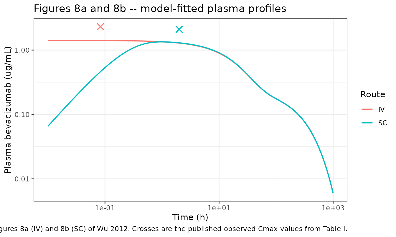
Figures 7 and 8c – draining axillary lymph node after SC dosing
Figure 7 shows the measured axillary-lymph-node concentrations after the SC dose (quantifiable only through 8 h) and Figure 8c overlays the model fit. The IV arm is included to show that the model reproduces the paper’s observation that lymph-node uptake after IV dosing is negligible – structurally, the model routes drug into the node only from the SC depot, so the IV node profile is identically zero.
sim |>
  dplyr::filter(time <= 24) |>
  ggplot(aes(time, Clnode, colour = treatment)) +
  geom_line(linewidth = 0.7) +
  labs(
    x = "Time (h)", y = "Lymph-node bevacizumab (ug/mL)", colour = "Route",
    title = "Figures 7 and 8c -- draining axillary lymph-node profile",
    caption = paste(
      "Replicates the model-fitted line of Figure 8c of Wu 2012 (data in",
      "Figure 7). Node uptake after IV dosing is structurally zero."
    )
  ) +
  theme_bw()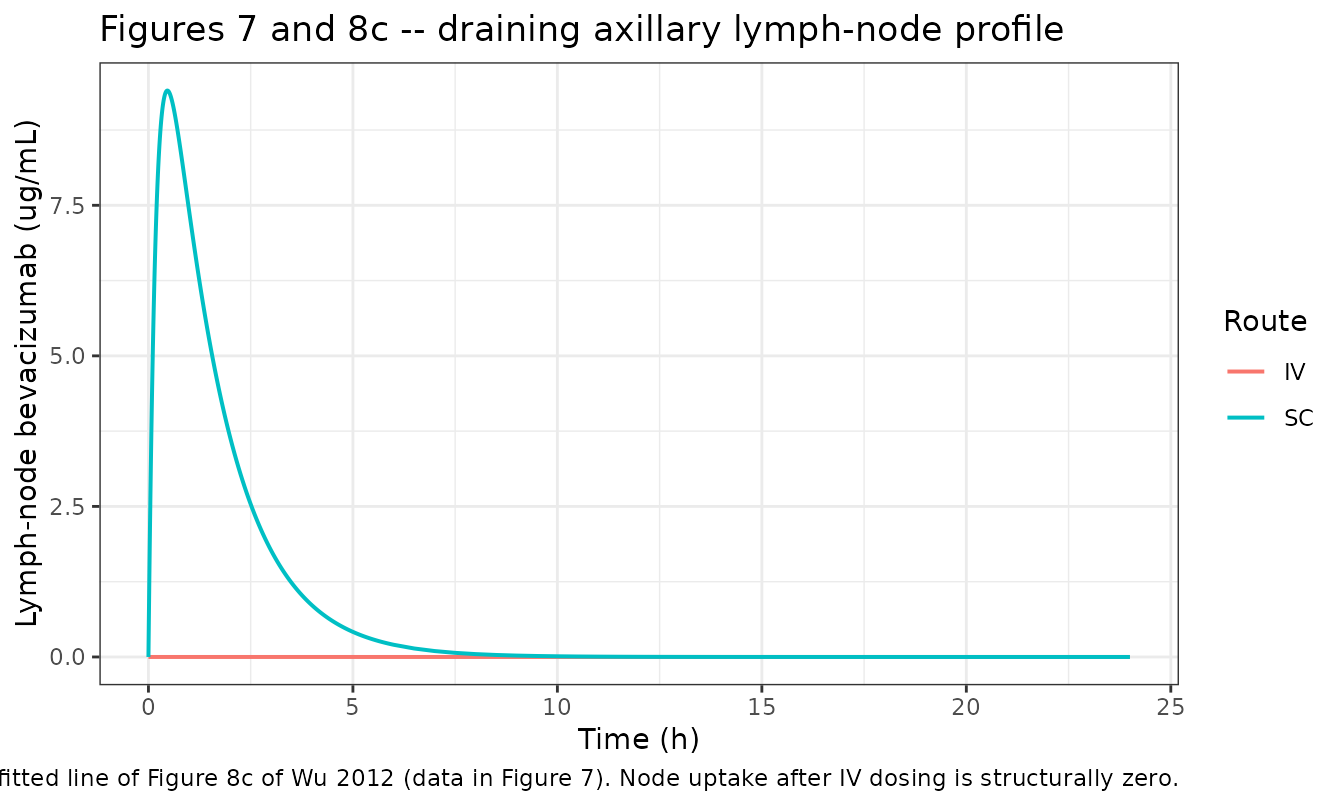
PKNCA validation
Plasma
sim_nca <- sim |>
  dplyr::filter(!is.na(Cc)) |>
  dplyr::select(id, time, Cc, treatment)

# Guarantee a time = 0 row per arm. Both arms already have one -- 0 for SC
# and the post-bolus Dose/Vc for IV -- and .keep_all keeps the existing row.
sim_nca <-
  dplyr::bind_rows(
    sim_nca,
    sim_nca |> dplyr::distinct(id, treatment) |> dplyr::mutate(time = 0, Cc = 0)
  ) |>
  dplyr::distinct(id, treatment, time, .keep_all = TRUE) |>
  dplyr::arrange(id, treatment, time)

conc_obj <- PKNCA::PKNCAconc(sim_nca, Cc ~ time | treatment + id)

dose_df <- events |>
  dplyr::filter(evid == 1) |>
  dplyr::select(id, time, amt, treatment)

dose_obj <- PKNCA::PKNCAdose(dose_df, amt ~ time | treatment + id)

intervals <- data.frame(
  start      = 0,
  end        = Inf,
  cmax       = TRUE,
  tmax       = TRUE,
  aucinf.obs = TRUE,
  half.life  = TRUE,
  cl.obs     = TRUE
)

nca_res <- PKNCA::pk.nca(PKNCA::PKNCAdata(conc_obj, dose_obj, intervals = intervals))
Lymph node (SC arm only)
The IV node profile is identically zero, so the node NCA is run on the SC arm alone.
The node window is truncated at 24 h. The node empties with a
half-life of log(2) / ka2 = 0.96 h, so by the end of the
plasma grid at 1000 h the node concentration has decayed below the ODE
solver’s absolute tolerance and takes small negative values; PKNCA then
fails to fit lambda.z and returns NA for
aucinf.obs. At 24 h – 25 node half-lives after the peak –
the profile is still strictly positive, and the extrapolated tail beyond
it is a part in a million of the total area.
node_nca <- sim |>
  dplyr::filter(treatment == "SC", time <= 24, !is.na(Clnode)) |>
  dplyr::select(id, time, Clnode, treatment)

# Guard the truncation: the window must stay clear of solver noise, or the
# mass-balance check below silently degrades instead of failing.
stopifnot(
  all(node_nca$Clnode >= 0),
  node_nca$Clnode[node_nca$time == 24] > 0
)

node_conc <- PKNCA::PKNCAconc(node_nca, Clnode ~ time | treatment + id)
node_dose <- PKNCA::PKNCAdose(
  dose_df |> dplyr::filter(treatment == "SC"),
  amt ~ time | treatment + id
)

node_res <- PKNCA::pk.nca(
  PKNCA::PKNCAdata(
    node_conc, node_dose,
    intervals = data.frame(
      start = 0, end = Inf, cmax = TRUE, tmax = TRUE, aucinf.obs = TRUE
    )
  )
)

node_val <- function(code) {
  x <- as.data.frame(node_res)
  v <- x$PPORRES[x$PPTESTCD == code]
  if (length(v) != 1L) stop("no unique node NCA row for '", code, "'")
  v
}
Comparison against published NCA
# Wu 2012 Table I. Table I reports no Tmax for the IV arm and no CL for the
# SC arm (the SC clearance is CL/F, which the paper does not tabulate), so
# those two cells are NA rather than fabricated.
published <- tibble::tribble(
  ~treatment, ~cmax, ~tmax, ~aucinf.obs, ~half.life, ~cl.obs,
  "IV",        2.31,  NA,     64.7,       93.8,       6.96,
  "SC",        2.10,  2.00,   91.4,      110.9,       NA
)

cmp <- nlmixr2lib::ncaComparisonTable(
  simulated = nca_res,
  reference = published,
  by        = "treatment",
  units     = c(
    cmax = "ug/mL", tmax = "h", aucinf.obs = "h*ug/mL",
    half.life = "h", cl.obs = "mL/h/kg"
  ),
  tolerance_pct = 20
)

knitr::kable(
  cmp,
  caption = paste(
    "Simulated (packaged model, typical value) vs. published NCA",
    "(Wu 2012 Table I). * differs from reference by >20%."
  ),
  align = c("l", "l", "r", "r", "r")
)| NCA parameter | treatment | Reference | Simulated | % diff |
|---|---|---|---|---|
| Cmax (ug/mL) | IV | 2.31 | 1.41 | -38.9%* |
| Cmax (ug/mL) | SC | 2.1 | 1.34 | -36.2%* |
| Tmax (h) | IV | — | 0 | — |
| Tmax (h) | SC | 2 | 0.99 | -50.5%* |
| AUC0-∞ (obs) (h*ug/mL) | IV | 64.7 | 87.1 | +34.6%* |
| AUC0-∞ (obs) (h*ug/mL) | SC | 91.4 | 87.1 | -4.7% |
| t½ (h) | IV | 93.8 | 185 | +97.7%* |
| t½ (h) | SC | 111 | 185 | +67.2%* |
| CL/F (mL/h/kg) | IV | 6.96 | 5.17 | -25.7%* |
| CL/F (mL/h/kg) | SC | — | 5.17 | — |
Seven of the nine comparable rows are starred. They are not seven
independent problems: they are three properties of the published fit,
each of which shows up in more than one row, and all three are discussed
under “Assumptions and deviations” below. In brief, the fitted
Vc is larger than the observed peaks imply (both
Cmax rows), the fitted terminal phase is flatter than the
observed decline (both t1/2 rows, and with it the IV
AUC and CL rows), and the fitted
ka1 is faster than the observed 2 h Tmax.
Nothing is tuned; Table II is transcribed as printed.
Two labelling notes on the table. ncaComparisonTable()
uses the package’s generic label CL/F for PKNCA’s
cl.obs; on the IV row that quantity is a true clearance,
not an apparent one. And the two dashes are cells Wu 2012 leaves blank –
Table I reports no IV Tmax and no SC clearance – rather
than values the model failed to produce.
Structural and mass-balance checks
These checks compare the model against itself and against quantities the paper states independently of the fit. Both sides of each check come from the same deterministic solve, so the residual is pure numerical-integration error and a tight bound is the correct assertion.
ui <- rxode2::rxode(mod)
par_val <- function(nm) {
  v <- ui$iniDf$est[ui$iniDf$name == nm]
  if (length(v) != 1L) stop("no unique ini() row for '", nm, "'")
  exp(v)
}
flnode  <- par_val("lflnode")
v_lnode <- par_val("lv_lnode")
k_ln_c  <- par_val("lk_lnode_central")
vc      <- par_val("lvc")
kel     <- par_val("lkel")

nca_wide <- as.data.frame(nca_res) |>
  dplyr::select(treatment, PPTESTCD, PPORRES) |>
  tidyr::pivot_wider(names_from = PPTESTCD, values_from = PPORRES)

get_nca <- function(arm, code) {
  v <- nca_wide[[code]][nca_wide$treatment == arm]
  if (length(v) != 1L) stop("no unique row for ", arm, " / ", code)
  v
}

# 1. Lymphatic mass balance. Every molecule that enters the node leaves it
#    for plasma, so the total amount transferred is
#      k_lnode_central * AUCinf(A_lnode) = k_lnode_central * v_lnode * AUCinf(Clnode)
#    and that must equal flnode * Dose exactly.
node_amount   <- k_ln_c * v_lnode * node_val("aucinf.obs")
node_fraction <- node_amount / dose_ug_per_kg

# 2. Bioavailability. BIO is fixed at 1 and Eqs. (3), (5) and (6) are
#    mass-conserving in BIO, so the SC and IV AUCs must be identical.
f_rel <- get_nca("SC", "aucinf.obs") / get_nca("IV", "aucinf.obs")

# 3. AUC identity. For a linear model AUCinf = Dose / (kel * Vc) on both arms.
auc_closed_form <- dose_ug_per_kg / (kel * vc)

checks <- tibble::tibble(
  Check = c(
    "Lymphatic fraction recovered from the node AUC equals Frc",
    "Bioavailability: AUCinf(SC) / AUCinf(IV) equals the fixed BIO = 1",
    "IV AUCinf equals the closed form Dose / (kel * Vc)",
    "SC AUCinf equals the closed form Dose / (kel * Vc)"
  ),
  Target   = c(flnode, 1, auc_closed_form, auc_closed_form),
  Achieved = c(
    node_fraction, f_rel,
    get_nca("IV", "aucinf.obs"), get_nca("SC", "aucinf.obs")
  )
) |>
  dplyr::mutate(`% diff` = (Achieved / Target - 1) * 100)

knitr::kable(
  checks, digits = c(0, 6, 6, 4),
  caption = "Internal identities of the deterministic solve."
)| Check | Target | Achieved | % diff |
|---|---|---|---|
| Lymphatic fraction recovered from the node AUC equals Frc | 0.00964 | 0.009640 | -0.0032 |
| Bioavailability: AUCinf(SC) / AUCinf(IV) equals the fixed BIO = 1 | 1.00000 | 0.999998 | -0.0002 |
| IV AUCinf equals the closed form Dose / (kel * Vc) | 87.07767 | 87.076699 | -0.0011 |
| SC AUCinf equals the closed form Dose / (kel * Vc) | 87.07767 | 87.076560 | -0.0013 |
# Deterministic: the only error here is trapezoidal integration and PKNCA's
# terminal extrapolation, so a tight bound is correct and will go red on any
# transcription slip in Frc, VLN, ka2, kel or Vc. The four rows realise
# -0.003%, -0.002%, -0.001% and -0.003%; 0.1% is ~30x headroom over that and
# still an order of magnitude below the smallest error a wrong digit in any
# of those five parameters could produce.
stopifnot(all(abs(checks$`% diff`) < 0.1))
The model’s lymphatic fraction, 0.964%, is also close to the paper’s
independent non-compartmental estimate of 0.85%,
obtained from the area under the node amount-time curve without any
compartmental fitting (Results). That is a genuine second, in-paper
target rather than a restatement of the fitted Frc.
# The independent estimate is a separate measurement, not an identity, so this
# bound is loose by design: it asserts the two agree to within a factor of 1.5,
# which is what "about 1%" versus 0.85% means, and still goes red on an
# order-of-magnitude transcription error in Frc.
stopifnot(
  node_fraction / 0.0085 > 1 / 1.5,
  node_fraction / 0.0085 < 1.5
)
Assumptions and deviations
No IIV and no residual error, because none is reported. The plasma and node data come from destructive sacrificial sampling (three animals per timepoint) and were fitted by naive pooling of Bailer-method means, so no between-subject variance component is estimable. The CV% column of Table II is the relative standard error of each point estimate, not a variance component, and is deliberately not encoded as IIV. Both residual SDs are
fixed(0); the model is deterministic. No variance was invented.-
BIO sits on the absorption rate, not on the dose. Equations (3), (5) and
- all multiply by
BIO: it appears once on the depot efflux term (dAsc/dt = -BIO * ka1 * Asc) and once on each of the two inflow terms. The system is therefore mass-conserving for any value ofBIO, andBIOscales the absorption rate rather than the absorbed fraction – which is not what a bioavailability parameter normally does. The equations are encoded exactly as printed (standing policy: when the text and the printed equation conflict, trust the equation). This is immaterial here because the paper fixesBIO = 1; the model file carries it as the canonicallfdepotso that the provenance and the fixed status are visible.
- all multiply by
The IV and SC equation sets are one system. The paper writes Eqs. (1)-(2) for the IV arm and Eqs. (3)-(6) for the SC arm, with identical disposition constants. The IV equations are the SC equations with an empty depot, so the packaged model encodes a single system: dose
centralfor the IV arm anddepotfor the SC arm. No information is lost.Per-kilogram normalisation. Table II reports
VcandVLNin mL/kg and the dose is given in mg/kg, so the model is coded per kilogram of body weight: state amounts are ug/kg, volumes mL/kg, and concentrations ug/mL. Simulating a specific animal simply means multiplying every amount by its body weight; the concentrations are unchanged.Known deviation 1 – the fitted model underpredicts both observed peak concentrations by about 40%. The model’s IV
C0isDose / Vc= 450 / 319 = 1.41 ug/mL against a published observed Cmax of 2.31 ug/mL, and the SC peak is 1.34 ug/mL against a published 2.10 ug/mL. The discrepancy is the same on both arms: the model reproduces the ratio of the two peaks (1.34 / 1.41 = 0.95 versus the observed 2.10 / 2.31 = 0.91) while placing both about 40% low, so it lives entirely in the fittedVc, which is correspondingly larger than the value the observed peaks imply. The simulated SC Tmax (about 1 h) is likewise earlier than the observed 2.00 h, which the fittedka1of 4.82 1/h (a depot half-life of 8.6 min) makes unavoidable. Table II is transcribed as printed; nothing is tuned.Known deviation 2 – the model reproduces the SC AUC but not the IV AUC, and that is the authors’ own point. The model’s clearance is
kel * Vc= 0.0162 x 319 = 5.17 mL/h/kg, soDose / CL= 87.1 h*ug/mL. That is within 5% of the published SC AUC (91.4) but 35% above the published IV AUC (64.7). A simultaneous IV + SC fit withBIOfixed at 1 has to split the difference between the two arms, and the Discussion says as much: “there may be differences in clearance between IV and SC, and this might be responsible for the higher AUC seen after SC administration of bevacizumab, compared with that after IV administration.” The published NCA IV clearance, 6.96 mL/h/kg, is 35% above the model’s 5.17 mL/h/kg for the same reason.-
Known deviation 3 – the fitted terminal half-life is roughly twice the published lambda-z half-life. The eigenvalues of the fitted disposition matrix are 0.0570 1/h (12.2 h) and 0.00373 1/h (186 h), and PKNCA recovers 185 h from the simulated profiles, against published lambda-z half-lives of 93.8 h (IV) and 111 h (SC) estimated from the mean curves over 72-288 h. The model’s terminal phase is therefore flatter than the observed decline, which is the other half of the AUC discrepancy above.
These three deviations are reported, not gated: the internal identities in the previous section are what the assertions test, because those are the checks that can actually detect a transcription error in this model.
No covariates. The paper reports none, and with 25-30 g inbred male mice dosed on a mg/kg basis there is nothing to scale.
Non-paper-derived parameter values: none. Every value in
ini()comes from Wu 2012 Table II or the Methods text, as recorded in the source-trace table above.