Tacrolimus (Woillard 2017)
Source:vignettes/articles/Woillard_2017_tacrolimus.Rmd
Woillard_2017_tacrolimus.RmdModel and source
- Citation: Woillard JB, Mourad M, Neely M, Capron A, van Schaik RH, van Gelder T, Lloberas N, Hesselink DA, Marquet P, Haufroid V, Elens L. Tacrolimus Updated Guidelines through popPK Modeling: How to Benefit More from CYP3A Pre-emptive Genotyping Prior to Kidney Transplantation. Front Pharmacol. 2017;8:358. doi:10.3389/fphar.2017.00358
- Description: One-compartment population PK model for immediate-release oral tacrolimus in the early period after cadaveric kidney transplantation (Woillard 2017), with two parallel gamma-distributed absorption routes (double-gamma absorption), first-order elimination and a dose-proportional steady-state trough offset C0. A three-level CYP3A metabolizer cluster (poor / intermediate / extensive, reconstructed inside model() from the recipient CYP3A5 expresser status and the CYP3A4*22 rs35599367 carrier indicator) acts as an ordinal power-model multiplier on the whole predicted whole-blood concentration. Fitted non-parametrically in Pmetrics and evaluated here in the closed form published by the authors, so the model describes ONE steady-state dosing interval.
- Article: https://doi.org/10.3389/fphar.2017.00358
Tacrolimus has a narrow therapeutic window and highly variable
pharmacokinetics, a large part of which is genetic. Woillard 2017 fitted
a non-parametric population PK model to 59 de novo cadaveric kidney
transplant recipients in order to turn CYP3A pre-emptive
genotyping into actionable starting-dose advice. The structural model is
the double-gamma absorption model of the Limoges group (Saint-Marcoux
2005, 2010; the same lineage as Debord_2001_cyclosporin and
Fromage_2025_mycophenolic_acid), and the only covariate
retained is a three-level CYP3A metabolizer cluster built from
CYP3A4*22 and CYP3A5*3.
Population
ui <- rxode2::rxode(readModelDb("Woillard_2017_tacrolimus"))
pop <- ui$population
tibble::tibble(Field = names(pop), Value = unlist(lapply(pop, as.character))) |>
knitr::kable()| Field | Value |
|---|---|
| species | human |
| n_subjects | 59 |
| n_studies | 1 |
| age_range | Mean 51.9 +/- 13.4 years (Table 1) |
| weight_range | Mean 70.4 +/- 13.9 kg (Table 1) |
| sex_female_pct | 64.4 |
| race_ethnicity | Not reported (single-centre Belgian cohort) |
| disease_state | De novo cadaveric renal transplant recipients, early post-transplant hospitalization period |
| renal_function | Creatinine clearance (Cockcroft-Gault) 60.1 +/- 20.0 mL/min at the PK course (Table 1) |
| dose_range | Immediate-release oral tacrolimus, initial dose 0.10 mg/kg body weight twice daily, then adjusted to trough concentration; dose before the PK course 5.5 +/- 2.7 mg (Table 1) |
| administration | Oral, twice daily |
| co_medication | Mycophenolate mofetil (81%) or mycophenolate sodium (19%) plus steroids on a standard tapering schedule. 21% received a P-glycoprotein inhibitor (atorvastatin, proton-pump inhibitors) at reduced dosage; no CYP3A inducer or inhibitor was documented. |
| genotype | CYP3A metabolizer clusters (Elens 2011 clustering, Results): 5 poor metabolizers (CYP3A53/3 carrying CYP3A422), 36 intermediate metabolizers (CYP3A53/3 not carrying CYP3A422) and 18 extensive metabolizers (CYP3A5 expressers not carrying CYP3A4*22). |
| regions | Belgium (single centre: Cliniques Universitaires Saint-Luc, Brussels) |
| notes | Prospectively recruited July 2007 - January 2009; the same cohort as Elens 2013 (Ther Drug Monit 35:608-616). Full 12-h PK profile in every patient before hospital discharge: pre-dose and 30 min, 1 h 30 min, 3, 4, 8 and 12 h after the morning dose, plus daily troughs. Tacrolimus measured in whole blood by chemiluminescent microparticle immunoassay (Abbott Architect). Target trough 10-20 ng/mL in week 1, 10-15 ng/mL thereafter. Estimation was NON-PARAMETRIC (Pmetrics NPAG), so the published typical values are means of the non-parametric marginal support-point distributions, not the parameters of a ‘typical subject’. |
Fifty-nine cadaveric renal transplant recipients were recruited prospectively at Cliniques Universitaires Saint-Luc (Brussels) between July 2007 and January 2009 and followed through their hospitalization (Table 1; the same cohort as Elens 2013). Immunosuppression was tacrolimus plus mycophenolate mofetil (81%) or mycophenolate sodium (19%) plus tapering steroids. Tacrolimus was started at 0.10 mg/kg twice daily and adjusted to trough, targeting 10-20 ng/mL in the first week and 10-15 ng/mL thereafter. Before discharge every patient had a full 12 h profile (pre-dose and 30 min, 1 h 30 min, 3, 4, 8 and 12 h after the morning dose), with whole-blood tacrolimus measured by chemiluminescent microparticle immunoassay (Abbott Architect).
The CYP3A clustering of Elens 2011 gave 5 poor metabolizers (PM; CYP3A5*3/*3 carrying CYP3A4*22), 36 intermediate metabolizers (IM; CYP3A5*3/*3 not carrying CYP3A4*22) and 18 extensive metabolizers (EM; CYP3A5 expressers not carrying CYP3A4*22).
# The cluster counts are reconstructible from the Table 1 genotype frequencies,
# which is what the model() reconstruction relies on: every *22 carrier was
# also a CYP3A5 non-expresser, and every CYP3A5 expresser was *1/*1 for CYP3A4.
star22_carriers <- 5L # Table 1: CYP3A4*1/*22 5 (8.5%)
cyp3a5_expressers <- 14L + 4L # Table 1: CYP3A5*1/*3 14 + CYP3A5*1/*1 4
n_total <- 59L
stopifnot(
  star22_carriers == 5L, # PM count in Results
  cyp3a5_expressers == 18L, # EM count in Results
  n_total - star22_carriers - cyp3a5_expressers == 36L # IM count in Results
)
Model structure
Absorption is the sum of two parallel gamma-distributed input routes (Supplemental Data 1),
disposition after a unit IV bolus is one-compartment, , and the authors give the analytic convolution of the two as the output equation of their Pmetrics model file,
with the regularised lower incomplete gamma function. Because the patients were at steady state, is the trough carried in from previous doses; it is dose-proportional (Table 2 footnote). The retained covariate multiplies the whole output,
with the CYP3A dummy taking the ordinal values PM = 0, IM = 1, EM = 2.
The packaged file stores the gamma components in the canonical transit parameterisation (, ) and stores as an apparent volume; the chunk below recovers the published numbers from the packaged ones.
theta <- setNames(ui$theta, names(ui$theta))
p <- list(
  a1 = exp(theta[["lntr1"]]) + 1,
  b1 = (exp(theta[["lntr1"]]) + 1) / exp(theta[["lmtt1"]]),
  a2 = exp(theta[["lntr2"]]) + 1,
  b2 = (exp(theta[["lntr2"]]) + 1) / exp(theta[["lmtt2"]]),
  r = exp(theta[["lfdepot"]]),
  vc = exp(theta[["lvc"]]),
  kel = exp(theta[["lkel"]]),
  C0 = exp(theta[["lrbase"]]),
  thCYP3A = theta[["e_cyp3a_cluster_cc"]]
)
p$FAIV <- 1000 / p$vc

# Round-trip against Table 2 (final model). These are exact recoveries of the
# printed values, not approximations, so the tolerance is numerical only.
stopifnot(
  abs(p$a1 - 12.33) < 1e-9,
  abs(p$b1 - 20.36) < 1e-9,
  abs(p$a2 - 15.19) < 1e-9,
  abs(p$b2 - 5.05) < 1e-9,
  abs(p$r - 0.46) < 1e-9,
  abs(p$FAIV - 24.52) < 1e-9,
  abs(p$kel - 1.52) < 1e-9,
  abs(p$C0 - 2.94) < 1e-9,
  abs(p$thCYP3A - 0.77) < 1e-12
)

tibble::tibble(
  Parameter = c("a1", "b1 (1/h)", "MAT1 (h)", "a2", "b2 (1/h)", "MAT2 (h)",
                "r", "F*AIV (ng/mL per mg)", "V/F (L)", "alpha (1/h)",
                "C0 (ng/mL per mg)", "theta_CYP3A"),
  Value = c(p$a1, p$b1, p$a1 / p$b1, p$a2, p$b2, p$a2 / p$b2, p$r,
            p$FAIV, p$vc, p$kel, p$C0, p$thCYP3A)
) |>
  dplyr::mutate(Value = round(Value, 4)) |>
knitr::kable()| Parameter | Value |
|---|---|
| a1 | 12.3300 |
| b1 (1/h) | 20.3600 |
| MAT1 (h) | 0.6056 |
| a2 | 15.1900 |
| b2 (1/h) | 5.0500 |
| MAT2 (h) | 3.0079 |
| r | 0.4600 |
| F*AIV (ng/mL per mg) | 24.5200 |
| V/F (L) | 40.7830 |
| alpha (1/h) | 1.5200 |
| C0 (ng/mL per mg) | 2.9400 |
| theta_CYP3A | 0.7700 |
Source trace
tibble::tribble(
  ~Quantity, ~Source,
  "v_abs(t) two-component gamma mixture", "Supplemental Data 1, equations 1-2",
  "I(t) = A_IV exp(-k t) one-compartment disposition", "Supplemental Data 1, equation 3",
  "C(t) closed-form convolution with P(n, x)", "Supplemental Data 1, equations 4-5",
  "C(t) = C(t)_TPV * theta_CYP3A^CYP3A", "Results, 'Covariate Analysis'",
  "a1 = 12.33 [6.25-18.41]", "Table 2, final model",
  "b1 = 20.36 [7.37-33.35] 1/h", "Table 2, final model",
  "a2 = 15.19 [9.46-20.91]", "Table 2, final model",
  "b2 = 5.05 [1.02-9.08] 1/h", "Table 2, final model",
  "r = 0.46 [0.40-0.51]", "Table 2, final model",
  "F*AIV = 24.52 [20.61-28.43]", "Table 2, final model",
  "alpha = 1.52 [1.19-1.85] 1/h", "Table 2, final model + footnote ('alpha = elimination parameter')",
  "C0 = 2.94 [2.42-3.47], dose-proportional", "Table 2, final model + footnote",
  "theta_CYP3A = 0.77 [0.74-0.80]", "Table 2, final model",
  "CYP3A cluster definitions (PM/IM/EM)", "Results, first paragraph (Elens 2011 clustering)",
  "Assay error polynomial SD = 0.0001 + 0.0762*C - 0.1433*C^2", "Methods, 'Pharmacokinetic Population Modeling'",
  "Gamma error multiplier = 0.43 (final model)", "Results, 'Covariate Analysis'",
  "Observed mean concentration-time profile", "Table 1",
  "Probability of target attainment by dose and cluster", "Table 3",
  "Baseline demographics and genotype frequencies", "Table 1"
) |>
knitr::kable()| Quantity | Source |
|---|---|
| v_abs(t) two-component gamma mixture | Supplemental Data 1, equations 1-2 |
| I(t) = A_IV exp(-k t) one-compartment disposition | Supplemental Data 1, equation 3 |
| C(t) closed-form convolution with P(n, x) | Supplemental Data 1, equations 4-5 |
| C(t) = C(t)_TPV * theta_CYP3A^CYP3A | Results, ‘Covariate Analysis’ |
| a1 = 12.33 [6.25-18.41] | Table 2, final model |
| b1 = 20.36 [7.37-33.35] 1/h | Table 2, final model |
| a2 = 15.19 [9.46-20.91] | Table 2, final model |
| b2 = 5.05 [1.02-9.08] 1/h | Table 2, final model |
| r = 0.46 [0.40-0.51] | Table 2, final model |
| F*AIV = 24.52 [20.61-28.43] | Table 2, final model |
| alpha = 1.52 [1.19-1.85] 1/h | Table 2, final model + footnote (‘alpha = elimination parameter’) |
| C0 = 2.94 [2.42-3.47], dose-proportional | Table 2, final model + footnote |
| theta_CYP3A = 0.77 [0.74-0.80] | Table 2, final model |
| CYP3A cluster definitions (PM/IM/EM) | Results, first paragraph (Elens 2011 clustering) |
| Assay error polynomial SD = 0.0001 + 0.0762C - 0.1433C^2 | Methods, ‘Pharmacokinetic Population Modeling’ |
| Gamma error multiplier = 0.43 (final model) | Results, ‘Covariate Analysis’ |
| Observed mean concentration-time profile | Table 1 |
| Probability of target attainment by dose and cluster | Table 3 |
| Baseline demographics and genotype frequencies | Table 1 |
Virtual cohort
The model carries no inter-individual variability (see Errata), so every simulated subject with the same genotype and dose has the same profile. The cohort is therefore one subject per (cluster, dose) cell: the three CYP3A clusters crossed with the five doses Woillard 2017 simulated in Table 3, plus the cohort’s mean pre-PK-course dose of 5.5 mg (Table 1).
clusters <- tibble::tribble(
  ~cluster, ~CYP3A5_EXPR, ~SNP_CYP3A4_RS35599367, ~level,
  "PM", 0, 1, 0,
  "IM", 0, 0, 1,
  "EM", 1, 0, 2
) |>
  dplyr::mutate(cluster = factor(cluster, levels = c("PM", "IM", "EM")))

doses <- c(2.5, 5, 5.5, 7.5, 10, 15)

# 0.02 h grid resolves Tmax (the peak is broad: MAT2 = 3 h) without an
# unnecessarily dense observation set.
obs_times <- seq(0, 12, by = 0.02)

arms <- tidyr::expand_grid(clusters, dose = doses) |>
  dplyr::mutate(id = dplyr::row_number())

make_rows <- function(a) {
  dosing <- tibble::tibble(id = a$id, time = 0, amt = a$dose, evid = 1L,
                           cmt = "depot")
  obs <- tibble::tibble(id = a$id, time = obs_times, amt = NA_real_, evid = 0L,
                        cmt = "depot")
  dplyr::bind_rows(dosing, obs) |>
    dplyr::mutate(
      cluster = a$cluster, dose = a$dose,
      CYP3A5_EXPR = a$CYP3A5_EXPR,
      SNP_CYP3A4_RS35599367 = a$SNP_CYP3A4_RS35599367
    )
}

events <- arms |>
  dplyr::group_split(id) |>
  lapply(make_rows) |>
  dplyr::bind_rows() |>
  dplyr::arrange(id, time, dplyr::desc(evid))

# Disjoint-ID guard: each subject belongs to exactly one (cluster, dose) cell.
stopifnot(
  nrow(dplyr::distinct(events, id, cluster, dose)) == nrow(arms),
  nrow(arms) == 18L
)
Observation rows carry cmt = "depot" because
depot is the model’s only ODE state; Cc is an
algebraic observable and rxode2 returns it as a column at those
rows.
Simulation
sim <- rxode2::rxSolve(ui, events = events, keep = c("cluster", "dose")) |>
  as.data.frame() |>
  dplyr::mutate(cluster = factor(cluster, levels = c("PM", "IM", "EM")))
#> Warning: multi-subject simulation without without 'omega'

stopifnot(!anyNA(sim$Cc), all(sim$Cc > 0))
Verification against the published equation
The first gate evaluates the published closed form independently in
base R with pgamma(); the second integrates the published
absorption rate against the published disposition function numerically.
Both are deterministic comparisons using the same parameter values, so
the tolerances are numerical, not statistical.
closed_form <- function(t, dose, level) {
  (p$C0 * dose +
     p$FAIV * dose * exp(-p$kel * t) *
       (p$r * (p$b1 / (p$b1 - p$kel))^p$a1 * pgamma((p$b1 - p$kel) * t, p$a1) +
          (1 - p$r) * (p$b2 / (p$b2 - p$kel))^p$a2 *
            pgamma((p$b2 - p$kel) * t, p$a2))) *
    p$thCYP3A^level
}

sim <- sim |>
  dplyr::left_join(dplyr::select(clusters, cluster, level), by = "cluster") |>
  dplyr::mutate(ref_closed = closed_form(time, dose, level))

err_closed <- max(abs(sim$Cc - sim$ref_closed))
stopifnot(err_closed < 1e-10)
gamma_density <- function(u, a, b) b^a / gamma(a) * u^(a - 1) * exp(-b * u)

conv_numeric <- function(t, dose, level) {
  if (t <= 0) {
    return(p$C0 * dose * p$thCYP3A^level)
  }
  integrand <- function(u) {
    (p$r * gamma_density(u, p$a1, p$b1) +
       (1 - p$r) * gamma_density(u, p$a2, p$b2)) * exp(-p$kel * (t - u))
  }
  area <- stats::integrate(integrand, 0, t, rel.tol = 1e-12,
                           subdivisions = 2000)$value
  (p$C0 * dose + p$FAIV * dose * area) * p$thCYP3A^level
}

conv_check <- sim |>
  dplyr::filter(dose == 5.5, time %in% c(0, 0.5, 1.5, 3, 4, 8, 12)) |>
  dplyr::rowwise() |>
  dplyr::mutate(ref_conv = conv_numeric(time, dose, level)) |>
  dplyr::ungroup()

stopifnot(nrow(conv_check) == 21L) # 3 clusters x 7 times; a zero-row check would pass vacuously
err_conv <- max(abs(conv_check$Cc - conv_check$ref_conv))
stopifnot(err_conv < 1e-8)
# 1. C0 is dose-proportional and is exactly the t = 0 concentration.
trough <- sim |>
  dplyr::filter(time == 0) |>
  dplyr::transmute(cluster, dose, per_mg = Cc / (dose * p$thCYP3A^level))
stopifnot(max(abs(trough$per_mg - p$C0)) < 1e-10)

# 2. The CYP3A effect is an exact power of theta_CYP3A at every time and dose.
ratios <- sim |>
  dplyr::select(time, dose, cluster, Cc) |>
  tidyr::pivot_wider(names_from = cluster, values_from = Cc) |>
  dplyr::mutate(im_pm = IM / PM, em_pm = EM / PM)
stopifnot(
  nrow(ratios) == length(obs_times) * length(doses),
  max(abs(ratios$im_pm - p$thCYP3A)) < 1e-12,
  max(abs(ratios$em_pm - p$thCYP3A^2)) < 1e-12
)

# 3. Abstract effect sizes: IM and EM concentrations relative to PM, with the
#    95% CI carried through from theta_CYP3A = 0.77 [0.74-0.80].
eff <- tibble::tibble(
  Cluster = c("IM vs PM", "EM vs PM"),
  `Reduction (%)` = round(100 * (1 - c(p$thCYP3A, p$thCYP3A^2)), 1),
  `CI95 (%)` = c(
    sprintf("%.0f-%.0f", 100 * (1 - 0.80), 100 * (1 - 0.74)),
    sprintf("%.0f-%.0f", 100 * (1 - 0.80^2), 100 * (1 - 0.74^2))
  ),
  `Published CI95 (%)` = c("20-26", "36-45")
)
stopifnot(identical(eff$`CI95 (%)`, eff$`Published CI95 (%)`))
knitr::kable(eff)| Cluster | Reduction (%) | CI95 (%) | Published CI95 (%) |
|---|---|---|---|
| IM vs PM | 23.0 | 20-26 | 20-26 |
| EM vs PM | 40.7 | 36-45 | 36-45 |
# 4. Mass-balance style identity: the dose-driven part of the AUC integrates to
#    F*AIV*D/kel over an infinite interval, independently of how the dose is
#    split between the two gamma routes. This is the analogue of
#    CL * AUCinf = F * Dose for this parameterisation.
auc_increment <- function(dose, level) {
  stats::integrate(
    function(t) closed_form(t, dose, level) - p$C0 * dose * p$thCYP3A^level,
    0, 200, rel.tol = 1e-10, subdivisions = 2000
  )$value
}
auc_chk <- tidyr::expand_grid(dose = c(2.5, 5.5, 15), level = 0:2) |>
  dplyr::rowwise() |>
  dplyr::mutate(
    numeric = auc_increment(dose, level),
    analytic = p$FAIV * dose / p$kel * p$thCYP3A^level
  ) |>
  dplyr::ungroup()
stopifnot(max(abs(auc_chk$numeric / auc_chk$analytic - 1)) < 1e-6)
The four gates are complementary rather than redundant: gate 1 fixes
the dose-scaling of C0, gate 2 the covariate exponent, gate
4 the absolute amplitude F*AIV and the elimination rate,
and the convolution gate fixes the absorption shape parameters that gate
4 is deliberately blind to (the AUC identity is invariant to how the
dose is split between the two gamma routes and to their rates).
Replicate published figures
# Replicates Figure 5 of Woillard 2017: predicted concentration-time profiles
# for one CYP3A poor, intermediate and extensive metabolizer. The source shows
# individual Bayesian profiles; here the typical-value profiles are shown at
# the cohort's mean pre-PK-course dose of 5.5 mg (Table 1), with the observed
# cohort mean concentrations (Table 1) overlaid.
observed <- tibble::tibble(
  time = c(0, 0.5, 1.5, 3, 4, 8, 12),
  conc = c(11.3, 19.9, 26.0, 22.2, 17.4, 12.6, 10.6),
  sd = c(4.2, 11.7, 11.1, 5.5, 5.4, 4.6, 3.8)
)

sim |>
  dplyr::filter(dose == 5.5) |>
  ggplot(aes(time, Cc, colour = cluster)) +
  geom_line(linewidth = 0.8) +
  geom_pointrange(
    data = observed, inherit.aes = FALSE,
    aes(x = time, y = conc, ymin = conc - sd, ymax = conc + sd),
    colour = "grey30", size = 0.3
  ) +
  scale_colour_manual(values = c(PM = "#e31a1c", IM = "#6a3d9a", EM = "#1f78b4")) +
  labs(
    x = "Time after morning dose (h)", y = "Tacrolimus (ng/mL)",
    colour = "CYP3A cluster",
    title = "Figure 5 -- typical profiles by CYP3A cluster (5.5 mg)",
    caption = paste(
      "Replicates Figure 5 of Woillard 2017. Grey points are the observed",
      "cohort mean +/- SD from Table 1 (all clusters pooled)."
    )
  ) +
  theme_bw()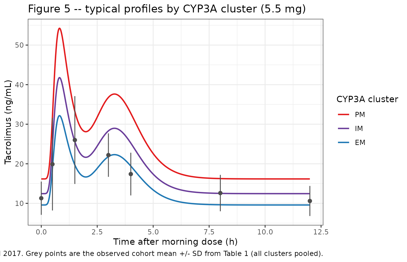
# Relates to Figure 6 / Table 3 of Woillard 2017: predicted steady-state trough
# by dose and CYP3A cluster, against the paper's 10-20 ng/mL week-1 target
# band. The source presents this as a probability of target attainment, which
# needs the non-parametric parameter distribution (not published); the
# typical-value trough is the deterministic counterpart.
sim |>
  dplyr::filter(time == 0) |>
  ggplot(aes(dose, Cc, colour = cluster)) +
  annotate("rect", xmin = -Inf, xmax = Inf, ymin = 10, ymax = 20,
           alpha = 0.12, fill = "#33a02c") +
  geom_line(linewidth = 0.8) +
  geom_point(size = 2) +
  scale_colour_manual(values = c(PM = "#e31a1c", IM = "#6a3d9a", EM = "#1f78b4")) +
  labs(
    x = "Dose (mg)", y = "Typical steady-state trough (ng/mL)",
    colour = "CYP3A cluster",
    title = "Typical trough by dose and CYP3A cluster",
    caption = paste(
      "Deterministic counterpart to Figure 6 / Table 3 of Woillard 2017.",
      "Shaded band is the paper's 10-20 ng/mL week-1 target."
    )
  ) +
  theme_bw()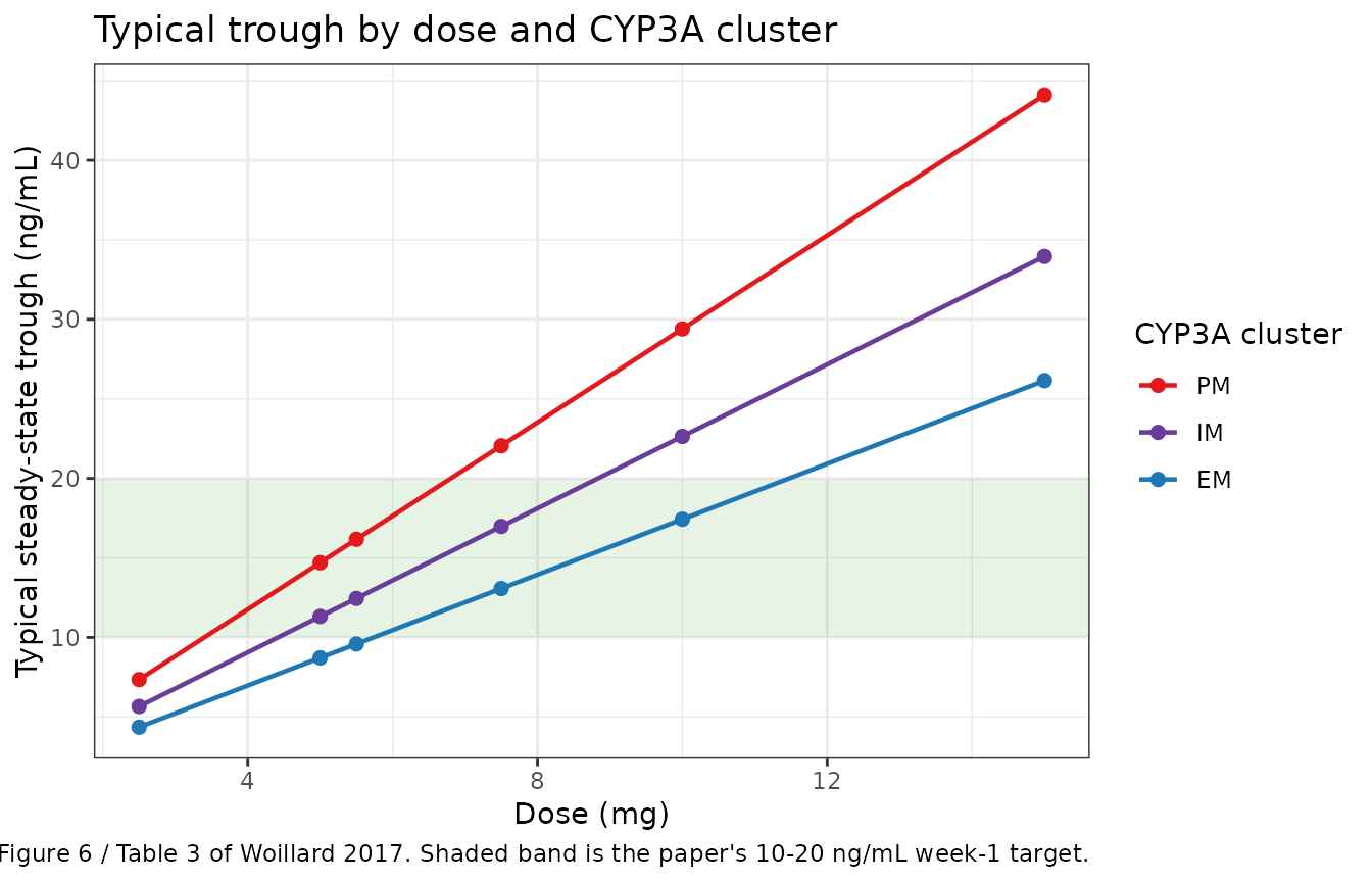
# Woillard 2017 Conclusion recommends 0.07 / 0.13 / 0.20 mg/kg b.i.d. for
# PM / IM / EM. At the cohort mean weight of 70.4 kg (Table 1) those are the
# doses below; the typical trough each produces is reported for reference.
wt <- 70.4
rec <- tibble::tibble(
  cluster = factor(c("PM", "IM", "EM"), levels = c("PM", "IM", "EM")),
  `mg/kg b.i.d.` = c(0.07, 0.13, 0.20)
) |>
  dplyr::mutate(
    `Dose at 70.4 kg (mg)` = round(`mg/kg b.i.d.` * wt, 2),
    level = c(0, 1, 2),
    `Typical trough (ng/mL)` =
      round(p$C0 * `Dose at 70.4 kg (mg)` * p$thCYP3A^level, 1)
  ) |>
  dplyr::select(-level)

# The paper's own recommendation is dose-escalating across PM -> IM -> EM; a
# sign error in the covariate exponent would invert this ordering.
stopifnot(all(diff(rec$`Dose at 70.4 kg (mg)`) > 0))
knitr::kable(rec)| cluster | mg/kg b.i.d. | Dose at 70.4 kg (mg) | Typical trough (ng/mL) |
|---|---|---|---|
| PM | 0.07 | 4.93 | 14.5 |
| IM | 0.13 | 9.15 | 20.7 |
| EM | 0.20 | 14.08 | 24.5 |
PKNCA validation
NCA is computed over the 0 to 12 h steady-state dosing interval.
cmin is used rather than ctrough; for this
model the time-zero concentration is the trough C0 * dose,
which the grid already contains.
# PKNCA reserves the column name `dose`, so the dose-level grouping column is
# carried as `dosegrp` on both the concentration and the dose object.
sim_nca <- sim |>
  dplyr::filter(!is.na(Cc)) |>
  dplyr::select(id, time, Cc, cluster, dosegrp = dose)

stopifnot(
  nrow(sim_nca) > 0,
  # Every subject must have a time-zero anchor or PKNCA warns per subject.
  nrow(dplyr::filter(sim_nca, time == 0)) == nrow(arms)
)

conc_obj <- PKNCA::PKNCAconc(sim_nca, Cc ~ time | cluster + dosegrp + id)

dose_df <- events |>
  dplyr::filter(evid == 1) |>
  dplyr::select(id, time, amt, cluster, dosegrp = dose)
dose_obj <- PKNCA::PKNCAdose(dose_df, amt ~ time | cluster + dosegrp + id)

intervals <- data.frame(
  start = 0, end = 12,
  cmax = TRUE, tmax = TRUE, cmin = TRUE, auclast = TRUE
)

nca_res <- PKNCA::pk.nca(
  PKNCA::PKNCAdata(conc_obj, dose_obj, intervals = intervals)
)

nca_wide <- as.data.frame(nca_res) |>
  dplyr::select(cluster, dosegrp, id, PPTESTCD, PPORRES) |>
  tidyr::pivot_wider(names_from = PPTESTCD, values_from = PPORRES) |>
  dplyr::mutate(cluster = factor(cluster, levels = c("PM", "IM", "EM"))) |>
  dplyr::arrange(cluster, dosegrp)

stopifnot(nrow(nca_wide) == nrow(arms), !anyNA(nca_wide$auclast))

nca_wide |>
  dplyr::rename(
    "CYP3A cluster" = cluster, "Dose (mg)" = dosegrp,
    "Cmax (ng/mL)" = cmax, "Tmax (h)" = tmax,
    "Cmin (ng/mL)" = cmin, "AUC0-12 (ng*h/mL)" = auclast
  ) |>
  dplyr::select(-id) |>
  dplyr::mutate(dplyr::across(dplyr::where(is.numeric), \(x) round(x, 2))) |>
knitr::kable()| CYP3A cluster | Dose (mg) | AUC0-12 (ng*h/mL) | Cmax (ng/mL) | Cmin (ng/mL) | Tmax (h) |
|---|---|---|---|---|---|
| PM | 2.5 | 128.53 | 24.66 | 7.35 | 0.82 |
| PM | 5.0 | 257.06 | 49.32 | 14.70 | 0.82 |
| PM | 5.5 | 282.76 | 54.25 | 16.17 | 0.82 |
| PM | 7.5 | 385.59 | 73.98 | 22.05 | 0.82 |
| PM | 10.0 | 514.11 | 98.64 | 29.40 | 0.82 |
| PM | 15.0 | 771.17 | 147.96 | 44.10 | 0.82 |
| IM | 2.5 | 98.97 | 18.99 | 5.66 | 0.82 |
| IM | 5.0 | 197.93 | 37.98 | 11.32 | 0.82 |
| IM | 5.5 | 217.73 | 41.78 | 12.45 | 0.82 |
| IM | 7.5 | 296.90 | 56.97 | 16.98 | 0.82 |
| IM | 10.0 | 395.87 | 75.95 | 22.64 | 0.82 |
| IM | 15.0 | 593.80 | 113.93 | 33.96 | 0.82 |
| EM | 2.5 | 76.20 | 14.62 | 4.36 | 0.82 |
| EM | 5.0 | 152.41 | 29.24 | 8.72 | 0.82 |
| EM | 5.5 | 167.65 | 32.17 | 9.59 | 0.82 |
| EM | 7.5 | 228.61 | 43.86 | 13.07 | 0.82 |
| EM | 10.0 | 304.82 | 58.49 | 17.43 | 0.82 |
| EM | 15.0 | 457.23 | 87.73 | 26.15 | 0.82 |
Tmax is the same in every cell because the model carries
no IIV and the covariate acts multiplicatively on the whole output, so
the profile shape is identical across clusters and doses. Note that this
Tmax is well before the paper’s second sampling time: the
peak comes from the fast gamma route and is narrow (see “Comparison
against published data” below).
Exposure is exactly dose-proportional within a cluster, which the model structure guarantees and the NCA output confirms:
Comparison against published data
Woillard 2017 reports no NCA table. The closest published exposure target is the observed cohort mean concentration-time profile of Table 1, measured at the cohort’s mean pre-PK-course dose of 5.5 mg. The model counterpart is the cluster-weighted mixture of the three typical profiles, weighted by the observed cluster sizes (5 PM, 36 IM, 18 EM).
weights <- c(PM = 5, IM = 36, EM = 18) / 59
mix_factor <- sum(weights * p$thCYP3A^c(0, 1, 2))

mixture <- sim |>
  dplyr::filter(dose == 5.5) |>
  dplyr::select(time, cluster, Cc) |>
  tidyr::pivot_wider(names_from = cluster, values_from = Cc) |>
  dplyr::mutate(Cc = weights[["PM"]] * PM + weights[["IM"]] * IM +
                  weights[["EM"]] * EM)

# The mixture is a scalar multiple of the PM profile because the covariate acts
# multiplicatively on the whole output; confirm the weighting is what we think.
stopifnot(max(abs(mixture$Cc / mixture$PM - mix_factor)) < 1e-12)
nca_from_profile <- function(df, label) {
  conc <- PKNCA::PKNCAconc(
    dplyr::mutate(df, id = 1L, src = label), conc ~ time | src + id
  )
  dose_d <- data.frame(id = 1L, src = label, time = 0, amt = 5.5)
  res <- PKNCA::pk.nca(PKNCA::PKNCAdata(
    conc, PKNCA::PKNCAdose(dose_d, amt ~ time | src + id),
    intervals = data.frame(start = 0, end = 12, cmax = TRUE, tmax = TRUE,
                           cmin = TRUE, auclast = TRUE)
  ))
  as.data.frame(res) |>
    dplyr::select(PPTESTCD, PPORRES) |>
    tidyr::pivot_wider(names_from = PPTESTCD, values_from = PPORRES)
}

# Reference: NCA of the Table 1 observed means, on the 7 published sampling
# times. Simulated: NCA of the cluster-weighted model mixture restricted to the
# SAME 7 times, so the trapezoidal rule sees an identical grid on both sides
# and the comparison is of the profiles, not of the sampling design.
ref_nca <- nca_from_profile(observed |> dplyr::select(time, conc), "observed")
sim_nca_mix <- nca_from_profile(
  mixture |>
    dplyr::filter(time %in% observed$time) |>
    dplyr::transmute(time, conc = Cc),
  "simulated"
)
stopifnot(nrow(ref_nca) == 1L, nrow(sim_nca_mix) == 1L)

cmp <- nlmixr2lib::ncaComparisonTable(
  simulated = sim_nca_mix,
  reference = ref_nca,
  params = c("cmax", "cmin", "auclast", "tmax"),
  tolerance_pct = 20,
  units = c(cmax = "ng/mL", cmin = "ng/mL", auclast = "ng*h/mL", tmax = "h")
)
knitr::kable(cmp)| NCA parameter | Reference | Simulated | % diff |
|---|---|---|---|
| Cmax (ng/mL) | 26 | 27 | +4.0% |
| Cmin (ng/mL) | 10.6 | 11.9 | +12.2% |
| Tmax (h) | 1.5 | 3 | +100.0%* |
| AUClast (ng*h/mL) | 192 | 214 | +11.3% |
# Gate on the numerics rather than on ncaComparisonTable()'s formatted
# character columns. Cmax, Cmin and AUC0-12 are compared; Tmax is recorded as a
# known deviation (see Errata) and is deliberately excluded from the gate.
pct <- function(nm) 100 * (sim_nca_mix[[nm]] - ref_nca[[nm]]) / ref_nca[[nm]]
exposure_pct <- vapply(c("cmax", "cmin", "auclast"), pct, numeric(1))
tmax_pct <- pct("tmax")

stopifnot(
  length(exposure_pct) == 3L,
  !anyNA(exposure_pct),
  max(abs(exposure_pct)) < 20
)

tibble::tibble(
  Metric = c("Cmax", "Cmin", "AUC0-12", "Tmax"),
  Observed = c(ref_nca$cmax, ref_nca$cmin, ref_nca$auclast, ref_nca$tmax),
  Simulated = c(sim_nca_mix$cmax, sim_nca_mix$cmin, sim_nca_mix$auclast,
                sim_nca_mix$tmax),
  `Difference (%)` = round(c(exposure_pct, tmax_pct), 1),
  Gated = c(TRUE, TRUE, TRUE, FALSE)
) |>
  dplyr::mutate(dplyr::across(c(Observed, Simulated), \(x) round(x, 2))) |>
knitr::kable()| Metric | Observed | Simulated | Difference (%) | Gated |
|---|---|---|---|---|
| Cmax | 26.0 | 27.05 | 4.0 | TRUE |
| Cmin | 10.6 | 11.89 | 12.2 | TRUE |
| AUC0-12 | 192.3 | 214.01 | 11.3 | TRUE |
| Tmax | 1.5 | 3.00 | 100.0 | FALSE |
The three exposure metrics agree with the published observed means to
within 12.2%, which is a meaningful check given that the model’s typical
values are non-parametric marginal means rather than a fitted typical
subject (see Errata). Tmax does not agree and is not
gated.
The comparison above is made on the paper’s seven sampling times on
both sides. That restriction matters, because at full
time resolution the model’s typical profile has a sharp early peak that
the published sampling grid cannot resolve: the fast gamma route carries
46% of the dose with a mean absorption time of 0.61 h and a width of
only 0.17 h (sqrt(a1)/b1).
full_res <- sim |>
  dplyr::filter(dose == 5.5, cluster == "PM") |>
  dplyr::slice_max(Cc, n = 1)

mixture_peak <- mixture |> dplyr::slice_max(Cc, n = 1)

# The true typical peak falls strictly between the 0.5 h and 1.5 h observed
# samples, so no published observation sits on it. This is deterministic (no
# IIV), so the bounds are structural, not statistical.
stopifnot(
  nrow(full_res) == 1L,
  full_res$time > 0.5, full_res$time < 1.5,
  # ... and it is materially higher than the value at either bracketing sample,
  # which is what makes the restricted-grid comparison the honest one.
  full_res$Cc > 1.3 * sim$Cc[sim$dose == 5.5 & sim$cluster == "PM" &
                               abs(sim$time - 1.5) < 1e-9]
)

tibble::tibble(
  Quantity = c("Typical Tmax, full resolution (h)",
               "Typical Cmax, PM at 5.5 mg (ng/mL)",
               "Typical Cmax, cluster mixture at 5.5 mg (ng/mL)",
               "Model value at the 1.5 h sample, mixture (ng/mL)",
               "Observed mean at 1.5 h (ng/mL)"),
  Value = round(c(full_res$time, full_res$Cc, mixture_peak$Cc,
                  mixture$Cc[abs(mixture$time - 1.5) < 1e-9],
                  observed$conc[observed$time == 1.5]), 2)
) |>
knitr::kable()| Quantity | Value |
|---|---|
| Typical Tmax, full resolution (h) | 0.82 |
| Typical Cmax, PM at 5.5 mg (ng/mL) | 54.25 |
| Typical Cmax, cluster mixture at 5.5 mg (ng/mL) | 39.90 |
| Model value at the 1.5 h sample, mixture (ng/mL) | 24.45 |
| Observed mean at 1.5 h (ng/mL) | 26.00 |
Consistency with the Table 3 probability of target attainment
Table 3 gives the simulated probability of exceeding each trough
target. Without the non-parametric parameter distribution the PTA itself
cannot be reproduced, but the PTA curve implies a
median trough per cell, and the ratio of the model’s
typical (mean) trough to that implied median is a check on the
C0 dose-scaling: for a right-skewed distribution with the
reported 40-80% CVs the ratio should be modestly above 1 and roughly
constant across cells.
# Table 3: P(trough >= target) for each (cluster, dose). Linear interpolation
# across targets gives the implied median (the target at which P = 50%).
pta <- tibble::tribble(
  ~cluster, ~dose, ~target, ~pct,
  "PM", 7.5, 2.5, 98.4, "PM", 7.5, 7.5, 91.7, "PM", 7.5, 10, 84.9,
  "PM", 7.5, 15, 60.8, "PM", 7.5, 17.5, 48.2, "PM", 7.5, 20, 38.6,
  "IM", 10, 2.5, 98.5, "IM", 10, 7.5, 91.2, "IM", 10, 10, 82.5,
  "IM", 10, 15, 61.0, "IM", 10, 17.5, 52.6, "IM", 10, 20, 45.7,
  "EM", 15, 2.5, 98.2, "EM", 15, 7.5, 87.0, "EM", 15, 10, 76.1,
  "EM", 15, 15, 58.8, "EM", 15, 17.5, 53.9, "EM", 15, 20, 47.6
)

implied_median <- pta |>
  dplyr::group_by(cluster, dose) |>
  dplyr::summarise(
    median_trough = stats::approx(pct, target, xout = 50)$y,
    .groups = "drop"
  ) |>
  dplyr::left_join(dplyr::select(clusters, cluster, level),
                   by = dplyr::join_by(cluster == cluster)) |>
  dplyr::mutate(
    typical_trough = p$C0 * dose * p$thCYP3A^level,
    ratio = typical_trough / median_trough
  )

stopifnot(nrow(implied_median) == 3L, !anyNA(implied_median$ratio))

# The ratio must be above 1 (a right-skewed distribution has mean > median) and
# consistent across the three cells. Read literally, the Table 2 footnote's
# "1000 mg" reference dose would put every typical trough three orders of
# magnitude below these medians, so this gate is what discriminates the two
# readings of that footnote (see Errata).
stopifnot(
  all(implied_median$ratio > 1),
  all(implied_median$ratio < 2),
  diff(range(implied_median$ratio)) < 0.5
)

implied_median |>
  dplyr::transmute(
    `CYP3A cluster` = cluster, `Dose (mg)` = dose,
    `Table 3 implied median trough (ng/mL)` = round(median_trough, 1),
    `Model typical trough (ng/mL)` = round(typical_trough, 1),
    `Ratio` = round(ratio, 2)
  ) |>
knitr::kable()| CYP3A cluster | Dose (mg) | Table 3 implied median trough (ng/mL) | Model typical trough (ng/mL) | Ratio |
|---|---|---|---|---|
| EM | 15.0 | 19.0 | 26.1 | 1.37 |
| IM | 10.0 | 18.4 | 22.6 | 1.23 |
| PM | 7.5 | 17.1 | 22.0 | 1.29 |
Assumptions and deviations
No inter-individual variability is encoded. The
paper reports only that “inter-patient variability in PK parameters was
represented by coefficients of variation ranging from 40 to 80% whereas
the correlation between parameters fluctuated from r = -0.497 to 0.410”
– a range over an unnamed set of parameters, with no per-parameter
variance and no covariance matrix. NPAG estimates a discrete joint
support-point distribution, which is not published either. Assigning
omegas from the 40-80% range would be an invention, so the packaged
model carries typical values only. The etas are omitted rather than
written as ~ fixed(0) because a zero-variance diagonal
makes OMEGA singular and breaks the Cholesky sampler used by
rxSolve(). A consequence is that the paper’s
probability-of-target-attainment analysis (Table 3, Figure 6) and its
VPC (Figure 4) cannot be reproduced; the deterministic counterparts are
shown above.
The C0 reference dose is read as 1000 ug, not
the printed 1000 mg. The Table 2 footnote defines
C0 as “the model estimated Tac trough level for a
theoretical dose of 1000 mg (the real trough level can be calculated by
dividing this value by 1000 and multiplying by the patient dose)”. Read
literally, the typical trough at the cohort’s mean 5.5 mg dose would be
2.94 / 1000 * 5.5 = 0.016 ng/mL, against observed troughs of 11.3 +/-
4.2 ng/mL (Table 1) and against Table 3, where 7.5 mg in a poor
metabolizer exceeds 10 ng/mL 84.9% of the time. Reading the reference
dose as 1000 ug = 1 mg gives C0 * dose[mg], a typical
trough of 16.2 ng/mL at 5.5 mg, and the typical-to-implied-median ratios
of the table above. It is also the only reading consistent with
F*AIV, which must use the same unit dose: per microgram it
would put V/F at 41 mL rather than 41 L.
Relatedly, the Table 1 row “Tac dose before PK course 5.5 +/- 2.7” prints no unit. It is taken as mg throughout this vignette, which is the only reading consistent with the stated 0.10 mg/kg twice-daily starting dose at the cohort’s mean weight of 70.4 kg (7.0 mg, subsequently titrated down to trough target).
The quadratic term of the assay error polynomial is
dropped. Methods gives
SD = 0.0001 + 0.0762*C(t) - 0.1433*C(t)^2 with a fitted
multiplier gamma = 0.43 for the final model. As printed, the quadratic
term drives SD negative above C = 0.53 ng/mL, i.e. across essentially
the whole observed range (the troughs alone are around 11 ng/mL), so the
coefficient has lost a power of ten that the paper does not supply. The
packaged model keeps the two usable terms – proportional 0.43 * 0.0762 =
3.28% and additive 0.43 * 0.0001 = 4.3e-5 ng/mL – and drops the
quadratic. The result is corroborated by the paper’s own fit
diagnostics: mean bias -0.11 +/- 3.7% and RMSE 4.5% (Results), both
consistent with a ~3.3% proportional residual.
The CYP3A cluster is reconstructed from two genotype
columns. Rather than registering a collapsed three-level
cluster column, the model takes CYP3A5_EXPR and
SNP_CYP3A4_RS35599367 as inputs and rebuilds the PM / IM /
EM level inside model(), per the convention documented in
the SNP_CYP3A4_RS35599367 entry of
inst/references/covariate-columns.md and following
MohammedAli_2023_tacrolimus.R, which reconstructs the same
Elens 2011 cluster from the same two inputs. The ordinal coding PM = 0,
IM = 1, EM = 2 is confirmed by the Abstract’s own effect sizes: 1 - 0.77
= 23% with CI [20-26%] for IM and 1 - 0.77^2 = 40.7% with CI [36-45%]
for EM, both intervals reproducing exactly. The Abstract prints “33%”
for IM, which is a typo – its own quoted interval [20-26%] does not
contain 33%, and 23% is what theta_CYP3A = 0.77 gives.
The peak shape is not reproduced, and Tmax is
not gated. At full time resolution the model’s typical profile
peaks at 0.82 h at 39.9 ng/mL for the cluster-weighted mixture at 5.5
mg, whereas the observed cohort means of Table 1 peak at 1.5 h at 26.0
ng/mL. Two distinct effects produce this, neither of them a
transcription error:
- The fast gamma route is a narrow pulse – shape
a1= 12.33 and rateb1= 20.36 give a mean absorption time of 0.61 h and a width (sqrt(a1)/b1) of 0.17 h – so the typical peak falls between the 0.5 h and 1.5 h sampling times and no published observation sits on it. - NPAG returns the means of the marginal support-point distributions, and the mean of a marginal is not the parameter vector of a typical subject. Feeding mean absorption parameters into the structural model produces a sharper, taller peak than the mean of the individual profiles, which is additionally flattened because subjects peak at different times.
The comparison against Table 1 is therefore made with the model
sampled at the paper’s own seven times on both sides, where the
amplitude metrics (Cmax, Cmin, AUC0-12) agree to within 12.2% – the
check that would catch a mis-transcribed dose, volume or clearance.
Tmax is reported but excluded from the gate. A user who
needs the peak reproduced should be aware that the published typical
values are marginal means; the individual Bayesian posteriors that
Figure 5 of the source plots are not published.
Single dosing interval only. tad() and
podo() refer to the most recent dose, so each dose restarts
the absorption input and there is no superposition. This matches the
authors’ framing – C0 is the steady-state trough
carried in from previous doses – but the model must not be used to build
up accumulation across doses.
Screened but unused covariates. Body weight, age,
sex, creatinine clearance, haematocrit, PPARA rs4253728,
POR*28 and the two ABCB1 SNPs were tested and not
retained. They are recorded in the model file’s
covariatesDataExcluded for provenance. Haematocrit and
PPARA were significant univariately (p = 0.0011 and 0.007) but
increased -2LL on inclusion; no point estimate is published for either,
so neither can be encoded even optionally.
Bioavailability is not separately identifiable.
Supplemental Data 1 states that “no independent estimation of the
bioavailability was possible because no intravenous data were available
for these patients”, so F*AIV is a product and the packaged
V/F is an apparent volume.
Erratum search. No erratum, corrigendum or author correction to doi:10.3389/fphar.2017.00358 was found on the Frontiers article page or in PubMed / EuropePMC at the time of extraction.